- explore Reaction-Diffusion as a form making system. what is the space of forms that it can create? what are the potential applications of this set of systems?
- learn to work with a complex simulation using reaction-diffusion as an example.
- produce a design using RD and fabricate it
Reaction-Diffusion workshop
Workshop Goals
Topics
- PDE solving techniques
- Forward Euler Finite Difference
- Matrix version of FEFD
- Implicit solvers
- Mesh laplacian
- adding one more dimension to other methods gives us 3D!
- notes: multigrid, FEM, on the GPU
- Control techniques
- different reactions
- Gray-Scott
- Fitzhugh-Nagumo
- Gierer-Meinhardt
- Brusselator
- lots more (oregonator, Turing)
- different starting conditions.
- anisotropic parameters
- anisotropic diffusion
- changing scale
- different reactions
- Realization techniques
- outlines / blob detection
- offsetting or thickening (could map to other surface)
- using time as 3rd dimension + marching cubes
- using it as parameter for some other solid system
- 3d reactions + marching cubes need to add full anisotropy
- other ideas?
- Advanced ideas
- multiple reactions on top of and interacting with each other
- reactions on a growing surface
- Reaction-Diffusion in Reality
Examples
download examples
- Different reactions
- reaction_diffusion_2d_basic
Gray-Scott
- reaction_diffusion_2d_brusselator
the Brusselator
- reaction_diffusion_2d_gm
Gierer-Meinhardt
- reaction_diffusion_2d_fhm
Fitzhugh-Nagumo
- reaction_diffusion_2d_basic
- Making things
- reaction_diffusion_2d_outline
using blob detection to create vector drawing of RD (uses blob detection library)
- reaction_diffusion_2d_time
create a voxel space with time as the 3rd dimension and extract isosurface with toxilibs volumeutils
- reaction_diffusion_mesh
using information from a RD simulation to modulate a mesh
- reaction_diffusion_3d_thicken
create a thick surface from the isosurface of a 3d RD simulation
- reaction_diffusion_2d_outline
- Simulation Techniques
- reaction_diffusion_2d_basic
simplest implementation of Central Difference Explicit Solver
- reaction_diffusion_2d_gm
using matrix notation to represent laplacian (uses mtj library)
- reaction_diffusion_2d_anisotropic
fully anisotropic 2d reaction variable direction and magnitude
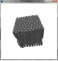
- reaction_diffusion_3d_anisotropic
- reaction_diffusion_mesh
use a mesh laplacian to solve RD directly on a surface
- reaction_diffusion_2d_basic
Reaction-Diffusion in nature
Reaction-Diffusion is a mathematical model of a theorized mechanism for biological pattern formation.
animal markings
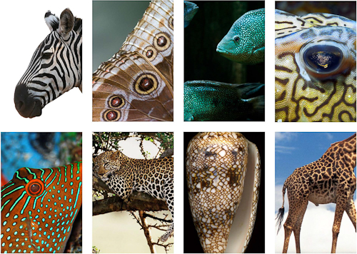
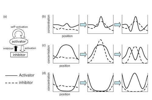
local amplification, lateral inhibition
Slide Mold aggregation
Reaction-Diffusion in art + design
Diffusion
the Laplace Equation
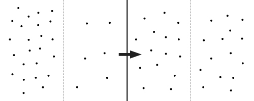 Diffusion is a passive spreading or averaging process. We think of it when we place a drop of dye in water or heat evens out in a room. More rigorously we can describe it as the motion en masse of particles moving randomly in a fluid. Here randomly means that the movement of a particle is independent of its previous state at any point in time, unlike Newtonian particles whose movement is dominated by forces and inertia. We are not concerned about the movement of an individual particle, but the aggregate motion of all the particles.
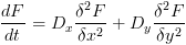
Mathematically, we use Partial Differential Equations (PDEs) to describe the dynamics of continuous quantities through space. This gives us a relation between how quantities change relative to their neighborhood. Statistical mechanics gives us a PDE which describes diffusion called the Laplace equation.
This equation states that the change of some quantity equals the laplacian (the triangle squared symbol) of the quanitity. The laplacian refers to sum of the second derivatives in each dimension, where the second derivative can be interpreted as curvature.
What this essentially says if the current position is more trough shaped, increase, if the current position is more crest shaped, decrease. In other words, the concentration goes towards the surrounding concentration. Over time in a closed system it averages out the concentration.
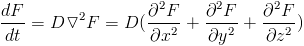
Computers work with discrete quantities, so to use these differential equations we need to convert them to regular equations of discrete quantities. We must create discrete versions of both space and time. There are several ways of doing so, and the simplest is called Finite Differences.
We divide space into a regular grid of points each point containing some concentration. Now we define a discrete version of differential operators based on a point and its neighbors. We can derive this is several ways the simplest being Taylor expansion.
This gives us a "stencil" which we can apply to each point of our grid to compute the Laplacian. The 5-point stencil shown above is the simplest version of a discrete laplacian. We apply the stencil by multiplying each value by its corresponding local grid point and summing them together. In matrix syntax this process is sometimes called convolution.
Explicit Integration (in time)
Finite difference gives us the right side of the Laplace equation, but we still have to deal with the left side: change in time. There are several methods or solvers for integrating in time. We will start with the simplest called explicit or forward Euler. This is based directly on the definition of the derivative:
Except since we are working with computers, we cannot work with continuous numbers, so instead of the limit as h goes to zero, we take h equal to some small value that we call
 . So to compute the value at the next time step, we take the current time step and add the derivative at the current time step multiplied by our time step.For 2D diffusion we get:
This is the simplest and easiest to implement type of integration. However, it is often error prone and unstable as we will see when we play with examples. Often the time step has to be kept very small.
****let's try to code diffusion****
other discretizations
There are many other ways to discretize space and integrate time. Finite difference defines differential quantities based on points. You can also choose different perspectives, such as looking at each square of the grid as a volume containing concentration. This is a type of "finite volume" approach and leads to slightly different equations. Finite element methods define "elements", which are often regions defined by a set of points. We then solve the equation for each element and stitch the elements together by their shared points.
Many integration techniques have been developed to deal with problems like error and stability. Backward or implicit integration uses the derivative at the next time step instead of the current one. This is more stable, but harder to solve. There are "higher order" methods that reduce error either by using previous time steps or by doing multiple integrations per step. You can also use a variable time step, to stay below a certain error threshold.
Laplacian applications
The Laplacian comes up in many different situations, not just Reaction-Diffusion. Understanding how to use and simulate this type of process has many applications
Heat transfer


 A prototypical engineering problem is to find the temperature of some element given the heating conditions. This amounts to solving the heat equation which looks exactly like the diffusion equation. This leads us to the problem of boundary conditions. For instance, in one dimension we want to know what the temperature of a bar is if we are keeping one side at a constant temperature and the other side is cooling at a constant rate. Or how fast does it heat up if one side is insulated. We have to figure out how to define these conditions mathematically and then how to implement them in our simulation. In more than one dimension, we can start to make more complex boundary conditions that are non-rectilinear or change in space and time.
Dielectric Breakdown Modeling
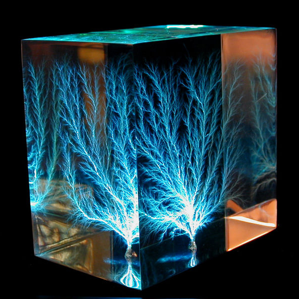
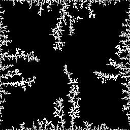
Dielectric breakdown modeling is trying to simulate something like formation of lighting. There is a dielectric or electrically insulating medium, like air, which is being ionized (broken down) by an electric field. The ionized medium is now a conductor going to ground, meaning the electric field at the conductor is zero. To compute the electric field, we use the diffusion equation. The ionized portions are a boundary condition held at zero. We can define the source of our electric field as a boundary held at one. We can simulate this process using the same technique to solve diffusion. The simulation progresses by ionizing areas with a stronger electric field. The steps of the simulation are as follows.
- initialize the simulation with a starting aggregation or ionized portion and boundary conditions
- compute the electric field using the diffusion equation
- ionize points next to the current aggregation with a probability proportional to the electric field
- repeat steps 2 and 3
Shape modeling
The laplacian has become a common tool in computer graphics. One application is to use the laplacian to encode the curvature of a surface. By representing the surface by its laplacian, we can recreate the surface holding certain points in fixed positions. This provides a way to modify a surface by pulling arbitrary points while maintaining the general shape.
Reactions
The other component to RD systems is the reaction. This is encoded as an ordinary differential equation, specifying a rate of change for a concentration. It does not depend on space making it somewhat simpler to simulate than the diffusion component
isotropic diffusion
uniform anisotropic diffusion
There are many possible reaction equation, which people are still inventing and modify. Some are based on real or hypothetical chemical reactions. Any system of chemical reaction can be turned into a differential equation. Others have been derived from population dynamics or equations for nerve cell potentials. Here are some commonly used reactions:
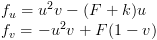
Gray-Scott:
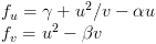
Gierer-Meinhardt:
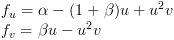
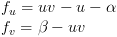
Brusselator:
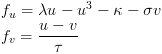
Fitzhugh–Nagumo:
Turing:
Each of these sets of equations has two chemicals "u" and "v". This is common for RD systems, though you can have more chemicals. Every other symbol in the equation is a parameter that you can vary. These parameters often represent something like the rate of decay of a chemical or an amount of chemical that is constantly being produced. One of the keys to using reaction diffusion is understanding how changing these parameters changes the resulting pattern. This can be difficult and often there is only a narrow range in which the RD system does anything at all.
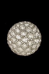
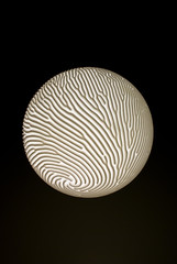
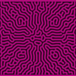
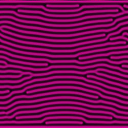
Changing parameters moves between different types of pattern. There are three basic types of patterns that most RD equations produce: dots, lines and an inverted dots pattern or polygons. We can give each cell of our grid different parameters, thus changing the pattern through space.
To get a sense of what parameters make which patterns, we can also make a parameter space simulation, where each axis represents a parameter which we smoothly change from one value to another.
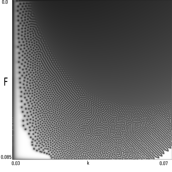
Here we have a Gray-Scott simulation where we are varying F from 0.0 to .085 and k from .03 to .07
Diffusion rates
The ratio of the diffusion rates is also very important to pattern formation. We said before that in an activator-inhibitor system that the inhibitor had to diffuse faster than the activator. Some systems have a ratio of 1:4; others have close to 1:100. This is another area where care is needed.
Anisotropic diffusion
isotropic diffusion
uniform anisotropic diffusion
So far, we have been describing systems with isotropic diffusion, where the diffusion rate is the same everywhere in every direction; however this does not necessarily have to be the case. The simplest form of anisotropic diffusion is having different diffusion rates in the x and y directions. In our diffusion equation that looks like:
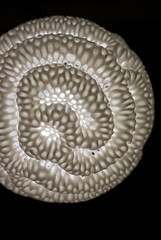
Additionally, these diffusion rates can change through space. Specifically, to create circular patterns, you can rotate the principle directions of diffusion around a point. We can talk more about that when we go over the examples
Initial conditions
Sometimes the initial conditions can effect the resultant pattern. A certain starting point might lead to a blank pattern where everything is the same while another leads creates highly differentiated forms. Often the pattern will grow off of certain initial shapes.
Realizations
blob detection to get outlines
heightmap
time as 3D dimension + isosurface
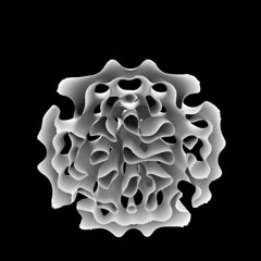
3D reaction-diffusion
heightmap
time as 3D dimension + isosurface
3D reaction-diffusion
Final Assignment
Design three 3d-printable cups using reaction diffusion.
The three designs must be substantially different from each other.
The maximum dimensions of each cup are 6x6x8cm. Your minimum wall thickness is 1.6mm (thicker is fine, but thinner designs may be too fragile). Consider adding a handle, base or other functional features to your cup.
We will meet with you via Skype on Tuesday at 4pm for a critique of your projects. Please prepare explanatory diagrams that show how you created the forms and share relevant portions of your code.
Possible ways to make a 3d-printable cup
- use the time extrusion sketch
- use 3d reaction-diffusion sketch
- use the mesh based reaction diffusion (if you use this you can only use it for one of your 3 cups)
To generate a cup shape with these methods you will have to find ways to constrain your reaction to a cup-like shape. For instance:
- changing f,K through space and/or time
- changing the diffusion rates through space and/or time
- changing the initial conditions
- remove concentration in certain locations to create a void
- distort a RD mesh (IN CODE)
Send us your questions and comments at hello AT n-e-r-v-o-u-s DOT com
Links
A technical explanation of diffusionFractal Dimension of Dielectric Breakdown
The Chemical Basis of Morphogenesis by Alan Turing
Reaction-Diffusion Textures by Andrew Witkins and Michael Kass
Advanced Reaction-Diffusion Models for Texture Synthesis - More RD for graphics
Meinhardt's website - Theoretical aspects of pattern formation
Examples from class
2d reaction-diffusion2d Anisotropic
time extrusion, 3D reaction diffusion, and mesh reaction-diffusion examples from class
Other Stuff
Introduction Slidesother Reaction-diffusion examples
Libraries
controlP5Peasycam
mtj matrix libraries
Blob detection