There are many ways of representing and drawing curves. At the simplest there are lines. In graphics, every curve is ultimately converted into lines when it is drawn. However, it is difficult to describe shapes as lines, it takes more memory and cannot be modified coherently. We need more abstract ways to represent curves.

Besides ellipses and rectangles, Processing has three built in ways to draw curves. The simplest is drawing lines. This can be done with the line command or using beginShape and vertex. We have already discussed how drawing lines or polylines can be disadvantages. Processing also has two methods for drawing curves. The bezier and bezierVertex draw what is called a degree three bezier curve. These use two end points and to control or handle points. The bezierVertex function only take three agruments and assumes you have already drawn the starting point, so it only takes to control points and an end point. The line between the end point and the control point specifies the tangent at the end point. If we string these together, it amounts to a curve that goes through the end points and with a specified tangent at each point. However, in order to appear smooth, we must be careful to make the tangents of neighboring beziers the same.

The other form of curve that processing supports natively is through the curve and curveVertex. These implement what are called Catmull-Rom splines, which we will discuss in more detail. This draws a smooth curve through the specified points. The curve command only supports four points, so to draw longer curves it is necessary to string several together or use curveVertex. The other caveat is that the first and last point of a curve only contribute to the tangent at the end points and do not get drawn. Commonly, this means that the first and last points must be repeated.

Often we want to go from a simple polygonal representation to a smooth curve. One method of doing so, which we will eventually generalize to surfaces, is called subdivision. This method takes a polyline and divides each line into two new lines, smoothing out the curve. By repeated applying this operation you get a smooth curve.

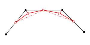
In more detail, for each segment of the polyline, you divide the segment in half. In other words, you make a new polyline that includes the midpoints of each segment. This gives us the same curve as before, just with more points. Then, the original points (not the midpoints) are moved to smooth out the curve. The only thing we need to know is where to move them. We want to move them inbetween their original positions and a position influenced by the midpoints. One way to think of this is to take the midpoint of the line between the new midpoints and use that as an approximation of the new point position. Then you average the original position and this approximation. Since the midpoints are just based on the original points, mathematically it is simple to describe the new point positions without referencing the midpoints.

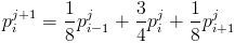
These weights give the smoothest results; however, we could play with them to get different results. For closed curves, it might look like this in code.

A parametric curve, in this instance, is a curve where each coordinate is defined by an independant function. Each of those functions is dependant on one variable, t. The curve is defined as all of the points defined by each t. So in equations we have.

To draw our curve, we simply iterate over t and draw a vertex for each evaluation of our function. The smaller the step, the closer our lines will approximate the curve. As an example, a spiral can be defined as

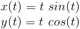
which looks like

Parametric curves are convenient because they are simple to define, write down, and play with. It is also relatively simple to find their tangents. You simply take the derivative of each component (on paper). However, they are not necessarily intuitive to manipulate because they are mathematically, not geometrically based. I have included a simple library to define parametric curves, with text-based equation, which you can download here.

Splines are the most common way of making curves in computer graphics and design. They are a specific type of parametric curve that is based on points.In so doing, they provide an intuitive, geometric way of defining curves. Unlike subdivision curves, which are also geometric, they can be evaluated exactly at any point, instead of discrete approximated by subdivision. The idea of splines is to take a set of points and use them to create separate polynomial curves that smoothly go together. The degree of the polynomial is the degree of the curve. For instance, we can interpret a polyline as a spline of degree 1. It is made up of separate lines (degree 1 polynomials), that are joined together to make a connected "curve".

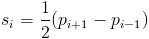
However, we want to make smooth curves. Most commonly, like all the default curves in Processing, people use degree 3 splines. Each degree of a curve can be interpreted as adding one degree of freedom. In our degree 1 case, each segment depends on two vector or end points. Phrased another way, we can draw a line between any two points. A degree 3 curves has two more degrees of freedom, so we can draw a degree 3 polynomial through any set of four points. However, our degrees of freedom do not have to be used as additional points, they can be any vector. For instance, instead of four points, we can specify to end points and the tangent each end point. From this, we get to the definition of Catmull-Rom splines, which is what Processing uses to draw curves.

We define a Catmull-Rom spline by taking a polyline and setting the tangent or slope at each point. There then exists a unique degree 3 polynomial between every pair of points. The tangents will match up where the separate polynomials meet, so it will appear smooth. The only questions left are how to the tangent at each point, and what is the exact form of the polynomial.

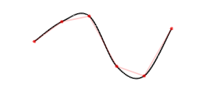
For a point p, we define the slope as half the next point minus the previous point. We can view this is the central approximation of the derivative at p

Now the polynomial between i and i+1 is

Or substituting in the points for slopes

For t between 0 and 1.

Often times it is desired to have more control over the shape of the curves, so it is possible to define a tension on each point. This is a scalar that we multiply the slope by. The higher it is the "tighter" the curve is. Sometimes it is also desired to normalize the slope by the distance between the points.

I will not go into detail here, but one of the most common representations in CAD is NURBS. It is a different way of defining a polynomial between each set of points and allows more flexibility than Catmull-Rom splines. NURBS stands for Non-Uniform Rational Bezier Splines. That sounds like a mouthful but we can break it down.

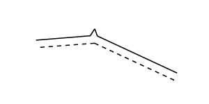
Non-Uniform means that the "parametric space" influenced by each point is variable. In the Catmull-Rom spline, the t is uniformly spaced between each point. It goes from 0 to 1. Or if we define it as a piecewise function, we could say it each segment goes from i to i+1. In NURBS, we can make this variable. We do so by defining what are called "knots". One of the most important roles that this plays is the ability to create cusps or sharp corners. By having the influence of point confined to a single parameter, we can create sharp corners.

Rational means we can assign a weight to each point. This is similar to the tension term in Catmull-Rom splines, but it is not applied to the slope. It is used whenever a point is used in computing the spline.

Bezier Spline refer to the fact that the polynomial that is being used is similar in form to bezier curves. This refers to the specific use of what are called Bernstein polynomials. However, the important information is that bezier splines do not interpolate the points of the curve. They act as "control points" influencing the curve but the curve does not pass through them like in Catmull-Rom splines.

The reason that NURBS are so important in computer graphics is because they are easy to evaluate, and they can represent a wide variety of specific shapes. For instance, by using certain weights, it is possible to create an exact representation of a circle. We can also represent curve with creases without having to represent them as two separate curves. This simplifies many operations because it does not require special cases for different types of curves. Everything can be represented by NURBS and treated the same: lines, ellipses, smooth curves, etc.

I have provided a basic NURBS library, which can be used to create NURBS curves and surfaces.

One of the most common operations you might want to do on a curve is offset it. It is often necessary to offset a curve for use with CNC machines. While doing a simple offset is easy, a robust offset that can accomodate complex shapes is very difficult. With complex forms, it can be better to use third party software, such as Adobe CS, to create offset curves.

In a simple case we can define an offset polyline by creating a new point for each vertex such that it is some distance from the segments that touch it. This can be done through a simple formula shown that can be seen geometrically:

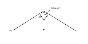
We can find the angle, a, between the vectors formed by those segments. We find the bisector of the segments by adding their normalized vectors. The distance along the bisector we find using the definition of the sin of angle. We can form a right triangle with the bisector, a segment, and a line of length d perpendicular to the segment. The distance along the bisector, d2, (hypotenuse) is d/sin(a/2). By adding our vertex and a vector along bisector of length d2, we get our new point. There are two problems we have to deal with: when we have a straight line and making sure we are offsetting to the correct side of our line.

However, this approach will not work on many curves. Any curves that intesect themselves will cause problems because the offset curves will overlap. More commonly, vertices can disappear in an offset because the offset distance is larger than the space between them.

Accordingly people have spent much effort developing robust offseting algorithms. One fairly easy way to get an approximate curve for an offset is using implicit surfaces. We define a function that it is greater than 0 within some distance d of the curve and less than 0 outside this area. We can then use a simple algorithm such as Marching Squares (the 2D version of Marching Cubes) to get the shape. This method will account for all degenerate cases, but it is computationally expensive and inexact. Depending on the application, you may also want to run a simplification/smoothing step afterwards to remove the stepping and straight segments from the results of marching squares.

To export curves there are two default options. The PDF export is good for 2D lines. For 3D, the only built in option is using the DXF export. The primary problem with the DXF export is that it is only supported with beginRaw. This means that instead of exporting the actual Processing commands, the output gets "processed" first. Specifically, curves and circles will be broken up into line segments and camera transformations will be applied. In other words, it is exporting what gets shown on your screen. Therefore, if you are using a camera, it is necessary to call camera() before you export to keep things where you expect them.

Making surfaces tends to be analogous to making curves only harder. Sometimes much harder. As all curves ultimately become lines, all surfaces ultimately become triangles. However, while maintaining a list of points to represent a polyline is trivial, maintaining a set of triangles is already a bit harder as a basic way to represent surfaces. Besides spheres and cubes, Processing does not provide any native methods to make surfaces except for triangles. These are created with the beginShape function, and you can look at that function for more details.

The simplest way to represent a surface is as a grid of points. Then we just draw a rectangle (which is two triangles) for each grid cell. This only works for surfaces that can be structured as a grid. This is the most direct analogy of our polyline. If a polyline is a one dimensional array of points, then a surface is a two dimensional array of points. Many surface methods, such as NURBS, are based on this type of representation. Often times, you want a more general way to represent a surface. These are generally called meshes.

There are many ways to represent a mesh. The simplest is just a list of faces and each face has an ordered list of vertices. However, this does not tell us any connectivity information. Often times you desire to know which faces are adjacent to each other or what faces a vertex belongs to. Also, each vertex belongs to multiple faces. For a compact representation and one that is easy to modify, you do not want that vertex to be stored separately in each face. Otherwise, you would have to modify every face to change one vertex. Creating good mesh representations not straight forward, so there are several methods ways to do it.

One common mesh structure is called a half-edge mesh. In this data structure, each edge is represented by two objects (half edges), one for each face that the edge borders. Half-edges are directed and the two half-edges that represent an edge (pair) point in opposite directions. Each half-edge (he) stores four pieces of information:

• The vertex at the end of the he
• The opposite pair he
• The face that includes the he
• The next he in the face

Each vertex only needs to store one he that contains it, and each face only needs to store one he that it contains. From there it is fairly straight forward to query adjacency information. For a good write of half-edge meshes, see this flipcode entry. There is also a half-edge mesh implementation for Processing by W:Blut but it is not particularly well documented as of yet. Two other mesh structure that are more general but more complicated are called radial edge and partial entity structures.

Just as we had subdivision curves, we can have subdivision surfaces. Unlike curves however, there are many ways we could imagine subdividing a surface represented by a mesh. The most common subdivision method is called Catmull-Clark. The idea behind this subdivision scheme is each face is divided into a new set of faces, one for each vertex.

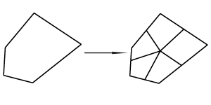
We determine the position for the point in the center of a face (face point) and the positions for the points that divide each edge in half (edge points). Then update the position of all original vertices.

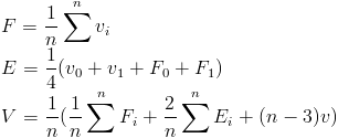
The face point equals the average of the vertices of that face. Each edge point equals the average of its end points and the face points of the adjacent faces. The new position of the vertex with n adjacent faces is the average of all the adjacent face points plus twice the average of all the adjacent edge points plus (n-3) times the previous position. This is normalized by dividing by n. In equation form

There are other types of subdivision schemes. The other most common one is called Doo-Sabin. For each face and vertex, it makes a new vertex, getting rid of the old vertices. This creates a new face for each vertex, edge, and face. The new vertices are created by a weighted average of the points of its face, .5 times the original vertex, .125 times the adjacent vertices, and 1/(4n) times all the vertices of the face (including the original and adjacent).

Though those two schemes are the most common, there exist many more. In fact, with these two as examples, you can sort of just start making them up. Some schemes have more limitations, such as only working on triangles. For open surfaces, you must modify all these schemes to account for boundaries.

Just like the with parametric curves, we can create parametric surfaces. The only difference is our functions have two variables instead of one. The same parametric utility from before has support for surfaces as well.

We can extend the idea of splines to surfaces fairly easy. Essentially, they are just like the curves except you do it more, in two directions. We do the spline operations in one direction and then another. Instead of a list of points, we have a two dimensional array of points

When we generalize Catmull-Rom splines to surfaces we get what is called bicubic interpolation. The spline was an implemenation of cubic interpolation, so when we do it twice it is called bicubic. We do cubic interpolation in one direction, which gives us a set of points to do cubic interpolation the other direction. Because cubic interpolation requires four points, the first step has to use cubic interpolation four times for the four points. It looks like this NURBS curves can be extending to surfaces in a similar manner. However, the power of this representation for surfaces in not in working with a 2D array of points, but being able to use more abstract surface construction methods. For instance you can loft multiple curves together to get a surface. The reason this is possible is due to a technique called knot insertion. This amounts to increasing the number of points used to represent a curve without changing the curve. This way you can take curves defined with different amounts of points, match them up, and use the resulting points as a new surface. We can also create other more complex surfaces such as swept, extruded, or revolved surfaces.

There are two common formats for 3D surfaces, obj and stl. Both are relatively simple formats. Both of these formats only support meshes, not curves or curved surfaces. STLs are the standard for rapid prototyping. They only support triangle, and consist of a list of triangles with some empty syntax around it. They look like a list of these statement with italics replaced with values:

facet normal nx ny nz
  outer loop
    vertex v1x v1y v1z
    vertex v2x v2y v2z
    vertex v3x v3y v3z
  endloop
endfacet
	    

OBJ files can support faces with an arbitrary number of faces. They also implicitly store connectivity information. Instead of storing each vertex with the face, first all the vertices are declared, then faces are defined by referencing the index of the vertices. The indices are determined by the order of the vertices starting with 1 (not 0 like arrays). An example of triangle would be:

v v1x v1y v1z
v v2x v2y v2z
v v3x v3y v3z
f 1 2 3
      

There are libraries to export OBJs and STLs, but sometimes they do not work as you would like. For instance, the superCAD library only support using beginRaw, which means if you want to export faces with more than three vertices it will not work.