This week will be devoted to introductions. First, we introduce the ideas and goals of the class. We also go over some of the basic mathematical concepts that will pervade most of the course. The focus is not on mathematical mastery or computation, but what we are calling scientific literacy. The goal is to be able to read and understand discourse in scientific disciplines. Finally, we will go over in detail a simple simulation.

• Introductions
• About this seminar
• Math
  • Vectors
  • Calculus
  • Linear algebra
• Diffusion limited aggregation
  • Basic implemenation
  • Optimizations
  • Interaction and extension

Click here to find tutorials and resources for mathematics.

We have a page to compile all the resources that everyone involved in the seminar has found that could be helpful or inspiring for projects.

Diffusion limited aggregation is a technique that attempts to simulate certain forms of growth. It is interesting in that it is both very simple and has broad applications to many diverse phenomena. It has been used to model coral, dendritic crystals, lightning, and snowflakes.

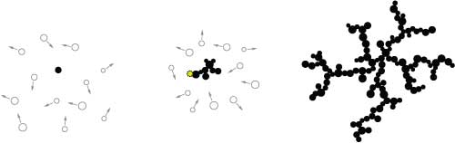
The premise is that you have particles moving randomly. This is called Brownian motion, which has an interesting history in its own right. When a particle hits a static structure, it sticks to it. In the most basic implementation, you start with a single fixed particle and add new particles in the manner described one at a time. The process naturally forms branches structures as the extremities of the growth act to block particles from hitting the interior parts of the static structure.

As our first project, we will look more indepth at different ways you might implement, interact with, and extend this system. We will also point to further resources where you can explore this topic in more detail. We start with a basic implementation and then show optimizations, extensions, visualization, etc.

There are two approaches to a basic DLA simulation. One works on a fixed grid and the other is grid-free and uses particles. This difference is reflected in many simulation techniques. Grids provide a rigid structure that simplifies the model. In this case, a particle can only move along the grid to one of its four neighbors. Working without a grid provides more freedom, but generally creates additional complexity, which can mean it is harder to program or requires more computation.

Here is the grid-free approach. Note that most of the work occurs in the addCircle function.

Here is the grid approach. If you run it note how the underlying grid structure effects the ultimate form. Note that you could run the simulation on any grid, though it would most likely require a slightly more complex data structure. You could even run it on arbitrary, irregular networks such as one formed from a voronoi diagram.

Generally, complex simulations will take a lot of computation, and depending on what you want to do with them speed can be an important factor. Therefore, optimizing your algorithm is often a necessary step. It is not usually necessary to talk about low level optimization, such as reducing function calls or using fast bit level operations, but higher level algorithmic optimizations are important to understand.

For instance, if you try to run the above grid-free code, essentially nothing with happen. This is because odds are as a particle moves randomly, it will move away from the existing aggregation and never return. So we want to make sure that the particle never moves too far away from the aggregation. This is accomplished by defining a circle around the aggregation that the particle must lay in. We can either have the particle wrap around when it hits the edge or have it "bounce" off. The code below shows the particle wrapping around. Here we have defined a vector called dla_center for the center of the aggregation, and bound_radius which equals the the radius of the circle that defines the maximum distance allowed from the center. It is necessary to keep track of the center of the aggregation and a radius which contains the aggregation as it grows. Please note that there are a number of other approaches to this problem including having a boundary box, bouncing off the boundary, or simply restarting the circle in a random starting location. The method shown is not necessarily optimal.

We can also increase the speed of the intersection part of the code. Notice that each time we try to find an intersection, we go through every circle in the aggregation. We call the time complexity of this function O(n), which means the number of operations grows linearly with number of circles. This can be reduced using a space partitioning algorithm, which means instead of checking every circle, we only check those that we know are nearby. This type of problem will come up in many different domains, and we will certainly come back to it in the future. There are many techniques developed for these problems. We will use the simplest in this case often called binning. We divide space into a grid of a regular size such that if a circle is in one grid square, it can only intersect with circles in a neighboring grid square. Because the number of possible neighboring circles is fixed, finding an intersection becomes a constant time function or O(1).

Once you have a system, you have to figure out how you want to use it. There are almost infinite directions you can take. This is the aspect in which you most directly act as a "designer". So what follows are merely some options of ways to interact with or develop the DLA system.

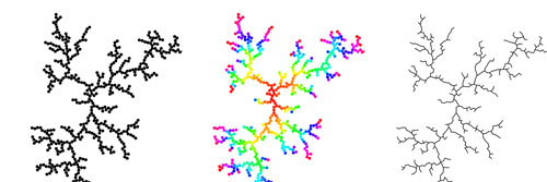We can identify some specific areas in the system we can explore to create variation. The most direct and superficial is how we visualize the aggregation. Often DLA patterns are drawn with the color of a particle corresponding to age. This gives a visual sense of how the structure grows. Another simple change is drawing the pattern as lines instead circles. This requires keeping track of the structure of which particles are intersecting. Other simple changes include varying the size of particles or extending the growth to more dimensions.

A property we can add to DLA is called stickiness. Instead of always sticking when a particle intersects, particles stick with some probability. By having a low probability, particles are able to slip past some of the exterior branching creating a denser pattern.

We can also change the environment in which the particles grow. The particles can stick to any initial starting surface. We can also confine the growth into a certain space.

Finally, the most rich area of variation is changing the way particles move. A simple directional force can be adding by making the particle tend in a certain direction as shown below. Going further, the particles can move in a force field. In the example presented in toxiclibs, a force field is created along a guide curve, sculpting the growth along a specified path. A force field could be created that responds to sound or video, so that the dynamics of the growth change through time. More advanced work studies what is called dielectric breakdown modeling, which attempts to simulate when an insulator breaks down and a spark jumps. In practice this is very similar to DLA except replacing the stochastic brownian motion with solving for the electric field, which is PDE formulation of the diffusion process. In essence, you are solving for the probability that a particle will hit any part of aggregation. In addition, you can manipulate the electric field by other means to effect or sculpt the growth. Some of the links on this page show work in this domain.

The first assignment is essentially to get start on your project. As a guide to starting, I recommend finding phenomena, projects, and papers you are interested in. You can use the inspiration page as a resource as well add things that you find to it. Compile a set of images, text, techniques, etc. that can be a starting point for your project. We can then discuss how you can approach the topics you have identified.