Particles are a powerful paradigm for simulation due to their simplicity. There are independent points whose position are updated according to some rules of dynamics. Many different systems are based on particles. You can simply have particles that move with some velocity and bounce off obstacles. Many agent-based models like flocking are essensially particle systems. You can also use particles to model continuum phenomena (smoothed particle hydrodynamics, which we will look at later). We will first look at classic point based mechanics. There are two basic components to this technique. First, computing trajectories based off position, velocity, and acceleration. This element is based on numerical methods for differential equations. The second component is computing the forces that determine acceleration. Classically in physics these forces are springs, gravity, electric fields, or in topics like atomistic modeling there are various approximate potential functions. However, these forces can be anything. They do not have to be based on physical principles or even normal physical space.
- Uses
- Particle System Structure
- Forces
- Springs and Gravity
- Energy and Fields
- Integrators
- Examples - Spring meshes

In physics, one of the standard examples of this technique is the
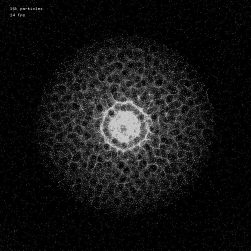
n-body problem, or many points acting with a gravitational force on one another. There is no analytic solution to this problem, so it has been a source of inquery for much of the history of physics and a natural candidate for computational methods. While this may be an interesting topic for physicists and astronomers, it is generally not that exciting for designers.
There is a long history of the use of particle systems in graphics. They are often used to simulate fake fluids, like smoke or water, as well as soft, deformable bodies like hair, cloth, or squishy blobs.
Visual effects or structures in design, such as Axel Kilian's CADenary project.
Forces are what you can use to control a particle system. There are basic forces which are implemented in many particle systems, such as springs and gravitational attractors. These forces are dependant on the relative positions of particles. There are also magnetic forces, which depend on velocity and position. We can also define our own forces, which can have almost any relation.
Springs are a restorative force. They attempt to keep two particles a certain distance apart. As an equation, the force looks like.

Where k is spring strength and  is the vector from one particle to another. We can look at a plot of the strength in one dimension here with Wolfram|Alpha
Gravitation or electrical forces drop off with distance squared.

With a gravitational force, the strength is also proporational to the mass of the particles.
Energy
Often, we think of things in terms of potential energy instead of force. Force is a vector, which points in a direction. Potential energy is a scalar. We can get from energy to force with the following equation.

The force equals the gradient of the energy. In other words, the force tries to "roll" down the potential energy hill. Often, it is easier to think in terms of energy because it is a scalar equantity. It can also be a powerful tool for analyzing systems because energy is conserved in a closed system. So instead of talking about defining different forces, we might talk about different potential functions. For instance, often in atomistic modeling, they use a function called the Lennard-Jones potential, which looks like C(a/r^12-a/r^6). This is convenient because it is easier to sketch out functions and have an idea of what they do. It is harder to draw or imagine vector fields in your head. Also, some more advanced integration techniques are derived from energy rather than force, though ultimately you get something similar.
The energy of a spring is

The energy of an attractor is

These forces are based on points, but we can also talk about general force or potential fields. For instance, a height map might be interpreted as a potential map instead. We can take a discrete representation, like an image, and turn it into a continuous representation through interpolation (going inbetween two values).
There is no need for the distance function d(a,b) = |(a-b)| to be sacred. We can imagine different distance functions that would also make our forces act differently. A simple example is simply eliminating a dimension, for instance having a force in 3D act in 2D. We might also try to have a force act in a kind of cylinder instead of rectilinear space. One might also try using city block distance or abs(x1-x2)+abs(y1-y2)+abs(z1-z2).
So how do particle systems actually work? You have a bunch of particles, each particle has a position and a velocity. There are also forces that determine the acceleration of particles. The approach to a lot of simulation problems is discretizing something that is continuous. In this case, we cannot determine where every particle is all the time because that is infinite. We would need an analytic solution that would give us the exact position at all times. Instead we chunk up time into finite time steps. What we want to determine is giving the positions, velocities, and forces in the current time step, what are they in the next time step. We do this using numerical integrators.
Integrators are numerical methods for solving differential equations. In general, with particle systems we are only solving one equation, which is the basic physics equation:

or in the form of a differential equation

Where x is the position vector.
There are many different integration methods. They tend to have names like Euler, Runge-Kutta, or other unhelpful names of people who are generally dead. Mostly, they are based off the same two ideas. The definition of the derivative:
and the Taylor approximation of a function:
Except since we are working with computers, we cannot work with continuous numbers, so instead of the limit as h goes to zero, we take h equal to some small value that we call  .
.
The simplest integrator is called the Euler integrator, but we can call it integrator number 1 or simple integrator. It takes the taylor approximation and truncates it to two terms, so it looks like this:
In code, that would look something like this:
Where velocity is the derivative of position, and acceleration, which is force/mass, is the derivative of velocity.
Error
In general, this method does not work very well. We can estimate the error of this method looking at the Taylor approximation. When we truncate the Taylor approximation the largest term that gets left out is multiplied by h^2. This means that if we halve our time step, our error is roughly one quarter. Note that this is a little deceptive because in order to perform the equivalent of a whole time step, we have to perform twice as many steps, leading to only having half as much error. This means that our total error is proportional to our time step,
, or O(h).
Other integration methods attempt to deal with the issue of error. There are two primary issues that concern us, how much error is there? This is similar to the above analysis. We also want to know how the error grows, which we refer to as stability. If the error gets larger and larger, we say it is unstable or it "blows up". Stability is dependant both on the integration method and what you are integrating. It is also more difficult to examine. The general idea is to look at the values you compute as the theoretical actual value plus an error term. You can then attempt to create an equation for how that error term changes every time your integrator takes a step.
Predictor-Corrector
There are many ways to "derive" some of the more complex integration schemes, manipulating the Taylor approximation or talking about fitting curve, and others. They form a couple basic regimes. One type is called predictor-corrector methods. In these methods you create an approximation of the next time step, using something like the Euler method, and then use that approximation to find an better result. However, in order to use the approximation, you have to re-evaluate your forces for those approximate positions and velocities. This is computationally equivalent to taking another time step. The simplest predictor-corrector method first makes an estimate of the derivative at the midpoint between the current time step and the next time step. Then it uses that estimate in a regular Euler step. The equation form might look like this:
and the code:
The most common predictor-corrector method is called Runge-Kutta of order 4. This is the default for the Traer.Physics library. It is similar to the method above, but uses recomputes the forces 4 times and has an error of O(h^4). You can look at the code for this method in the source for the library. In equations it looks like this.
Every call to f(t,x) represents recomputing the forces (expensive part).
I will also show another method that uses three previous time steps to make a better estimate. It has similar error characteristics to Runge-Kutta 4, but only requires two force computations called the Adams-Moulton method. As can often happen, you sacrifice memory for computation.
Implicit Methods
In the all the previous methods, you use the previous time steps to compute the value for a new time step. Another class of integrators instead computes an equation for the next time step, which then must be solved with another method. The advantage is that these methods are much more stable; however, they require the additional complexity of solving the system of equations. The simplest is a modified version of the Euler Method, often called the backwards Euler Method. Simply switch around the terms a bit you get:

Notice how we do not yet know the right side of the equation. To solve it either requires having an analytic function for the force or making a linear approximation. Look at
Baraff's lecture notes for more details. Ultimately, we must solve a sparse set of linear equations, which has its own set of methods for dealing with. Though complex, it can lead to drastically more stable simulations.
Variable steps and error estimates
Another method to prevent error is using a variable time step. The idea is use one calculation to estimate your current error, then change your time step to make sure your error is below a certain threshold. In a simple case you could compare taking two times steps of
, which we will call

versus one time step of

,

. With a method of error

, we can assume our error looks like

. We can estimate our error as

You can now choose a new time step that keeps your error within certain bounds. More advanced methods avoid taking all the extra steps (three instead of one), by computing two different integration methods at once that have different orders of error. For instance you could use the normal Euler method in conjunction with the mid-point method, since the Euler method is necessary to compute the mid-point method anyway. Similar techniques exist for the Runge-Kutta methods as well.
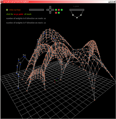
Examples - Spring meshes
One common use for particle systems is modeling soft, or deformable, bodies like cloth or the hanging chain models of CADenary. These methods use meshes of springs. The attached examples show several different uses of spring meshes.
The first example shows a grid of springs in 2D. We can use different types of forces to deform the mesh. We show some example custom forces. A spiral force is an attraction rotated 90 degrees.
The PotentialNoise force shows an example of a potential energy function defined by the noise function. We estimate the gradient of energy by discretely varying the noise function and use that as the force.