Diffusion is a passive spreading or averaging process. We think of it when we place a drop of dye in water or heat evens out in a room. More rigorously we can describe it as the motion en masse of particles moving randomly in a fluid. Here randomly means that the movement of a particle is independent of its previous state at any point in time, unlike Newtonian particles whose movement is dominated by forces and inertia. We are not concerned about the movement of an individual particle, but the aggregate motion of all the particles.
It is generally difficult to think about or describe random motion, but statistical mechanics gives us a partial differential equation which describes the evolution of the concentration of particles in space.
This equation essentially says if the current position is more trough shaped, increase, if the current position is more crest shaped, decrease. In other words, the concentration goes towards the surrounding concentration. Over time in a closed system it averages out the concentration.
This process and equation is seen in many contexts. In engineering, it is most commonly seen at the heat equation, which looks at how heat moves through space. We can also think of it in the motion of chemicals in solution. These two examples are the most analogous to the physical description of diffusion, but it also comes up in other situations. It can be seen in finacial modeling. A type of smoothing called laplacian smoothing is used in 3D mesh modeling. It is also a component of many other phenomena such as fluid motion.
Heat transfer
A prototypical engineering problem is to find the temperature of some element given the heating conditions. This amounts to solving the heat equation which looks exactly like the diffusion equation. This leads us to the problem of boundary conditions. For instance, in one dimension we want to know what the temperature of a bar is if we are keeping one side at a constant temperature and the other side is cooling at a constant rate. Or how fast does it heat up if one side is insulated. We have to figure out how to define these conditions mathematically and then how to implement them in our simulation. In more than one dimension, we can start to make more complex boundary conditions that are non-rectilinear or change in space and time.
Dielectric Breakdown Modeling
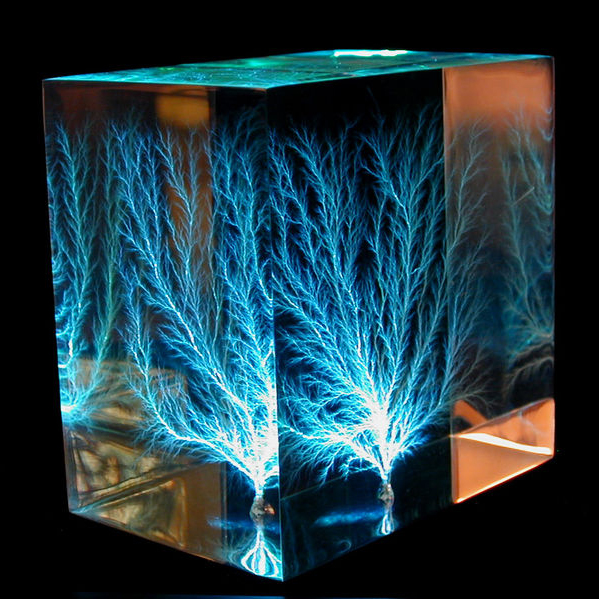
Now we can revisit dielectric breakdown modeling, which is a type of DLA-like growth. Dielectric breakdown modeling is trying to simulate something like formation of lighting. There is a dielectric or electrically insulating medium, like air, which is being ionized (broken down) by an electric field. The ionized medium is now a conductor going to ground, meaning the electric field at the conductor is zero. To compute the electric field, we use the diffusion equation. The ionized portions are a boundary condition held at zero. We can define the source of our electric field as a boundary held at one. This problem can be solved by the methods described below. The simulation progresses by ionizing areas with a stronger electric field. This method works on a grid, which is how we are solving our PDEs anyway right now. The steps of the simulation are as follows.
initialize the simulation with a starting aggregation or ionized portion and boundary conditions
compute the electric field using the diffusion equation
ionize points next to the current aggregation with a probability proportional to the electric field
repeat steps 2 and 3
Solving the diffusion equation can be a time consuming step, so the simulation proceeds very slowly. We can view this simulation as an analytic or continuous version of DLA. Instead of a stochastic process of moving a particle until it hits, we calculate the probability of a particle hitting any portion of the current aggregation. This gives us a more general and rigorous framework to think about this type of growth. We can more easily define specific "site conditions". If we make our equation more complicated, by adding advective, or flow, terms we can look at growth in a flowing medium, though this makes our simulation more complex.
Reaction Diffusion
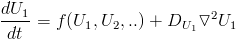
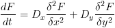
Making a fairly simple modification to the diffusion equation leads to one of the most powerful pattern generating systems in the natural world. This is a type of system called reaction-diffusion. The idea is to simulate one or more chemicals in diffusion and in addition these chemicals react with each other to change their concentration. So your equation has a diffusion component which is the same as above and a reaction component, which is an function dependent on the current chemical concentrations.
Where f is the reaction function.
There are a couple essential components to a reaction-diffusion system. The obvious one is the reaction functions for each reactant and the number of reactants. Many reaction systems have been proposed based off of chemical models as well preditor-prey population simulations and other areas. The less obvious component is the diffusion rates. Reaction diffusion systems only work with a specific ratio of diffusion rates between the chemicals. If both chemicals diffuse at the same rate, no pattern will form. Similarly if the rates are too different, nothing happens. One of the difficulties of working with reaction-diffusion systems is finding the right parameters for a given set of reaction equations, both diffusion rates and reaction parameters.
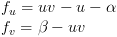
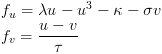
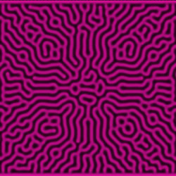
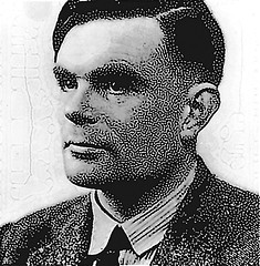
Reaction-diffusion is hypothesized as a common pattern formation mechanism in biological systems. Many animal patterns can be emulated with different reaction-diffusion equations. Interestingly the cuttlefish can change the pattern and color of its skin, and all of the patterns that it creates look like reaction-diffusion patterns. There are many different reaction-diffusion systems, and here we will show the reaction functions for a few. Alan Turing was first to propose reaction-diffusion as a model for pattern formation in biological system. One system he proposed looked like:
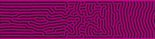
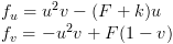
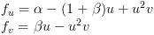
Another commonly used set of equations is called Gray-Scott:
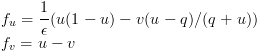
One of the only actual chemical reactions found that acts like a reaction diffusion system is called the Belousov-Zhabotinsky (BZ) reaction. When the proper set of chemicals is mixed together, it actually pulsates different colors. A simplified version of this is codified in the reaction diffusion system called Oregonator:
And some more.
Fitzhugh�Nagumo:
Brusselator:
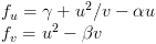
Gierer-Meinhardt:
While these are all two component systems, there are reaction-diffusion systems with more components. I only mention these systems to give: 1. search terms for more information and 2. a sense for the general form of these equations. One of the primary areas of study in reaction-diffusion systems is understanding when they are stable, oscillitory or degenerate. Basically people want to know under what conditions interesting patterns form, and by doing so get an understanding of why they form.
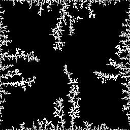
isotropic diffusion
uniform anisotropic diffusion
There are other ways to manipulate reaction-diffusion systems besides changing the reaction functions. The most common is to use anisotropic diffusion. So far, we have been describing systems with isotropic diffusion, where the diffusion rate is the same everywhere in every direction; however this does not necessarily have to be the case. The simplest form of anisotropic diffusion is having different diffusion rates in the x and y directions. In our diffusion equation that looks like:
Additionally, these diffusion rates can change through space. Specifically, to create circular patterns, you can rotate the principle directions of diffusion around a point. How that is done is explained in the linked papers on reaction-diffusion textures. You can also introduce inhomogeneity in other parameters.
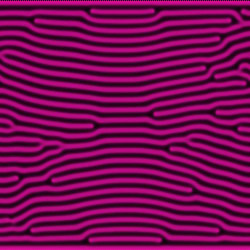
This image shows an experiment by Robert Hodgin (aka flight404) varying parameters of the Gray-Scott reaction by an image to create a stippling pattern.
Simulation - Finite Differences
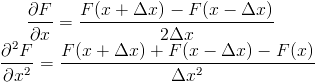
The simplest method for solving PDEs is called finite difference. Like ODE solvers which use finite versions of derivatives, this method uses finite versions of partial derivatives. So using a central difference, we can write a partial derivative as:
These show examples of what are called central differences, because the difference is centered around x as opposed to looking forward or backward in space. For a somewhat complete look at different difference approximations, see the wikipedia article
To solve these equations we discretize space and time. We can divide space into a grid with spacing and move forward in time with time steps of . We can employ several different difference approximations and integration methods to solve the PDE.
Explicit Methods
Just like with ODE solvers, there are many different approaches to PDE solvers that vary in complexity, efficiency, and stability. Explicit methods, similar to methods that we saw for particle systems, use the current time step to directly compute the next time step.
Forward Euler Central Difference
The most straight forward method to solve the diffusion equation uses simple Euler integration in time and central difference approximations in space. So the evolution of the system looks like:
and in code
Note this example uses periodic boundary conditions.
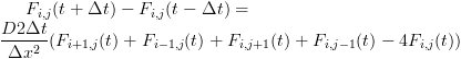
This method has limited stability. In fact, it can be shown that if is greater than .25, it will blow up. This limits the speed of the simulation since your time step will always have to be small. The error is also the same as the forward Euler method for ODEs.
Leapfrog / Dufort-Frankel
One modification that attempts to address this instability is using the central difference in time as well as space. Central difference has both more stability and less error in theory. This modification looks like this in the finite difference equation:
This is called the Leapfrog method as the next time step does not depend directly on the previous time step. Now, you must keep track of the previous time step as well as the current time step. It turns out that this is actually very unstable, but a slight modification leads to a method which is unconditionally stable for the diffusion equation.
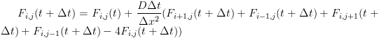
We replace every instance of the current point in space and time on the right side of the equation with the average of the next and previous time steps:
Now the simulation will remain stable regardless of the time step, however, the error in the simulation will still increase. Also, this only works for very specific differential equations. In code it looks like this:
Implicit Methods
As with particle systems, implicit methods use the derivative at the next time step instead of the current time step. While in particle systems this was a bit confusing since it we could not actually write down the force at the next time step, in this example it is much simpler. We write:
Crank-Nicholson
A slightly better method uses an average of the derivative at the current time step and the next time step. We can think of this as a midpoint approximation of the derivative. This is called the Crank-Nicholson method. Writing the implicit equation at each point in space gives us a set of linear equations. Each point depends on its four neighbors.
We now need to solve this set of equations. There are many methods for solving systems of linear equations efficiently, and I will only mention some of them now. You can directly solve them with Gaussian elimination or LU decomposition, however this tends to be prohibitively computationally expensive. The alternative is to use iterative methods. These include Gauss-Seidel relaxation and Conjugate Gradient. Many of these methods depend on this specific form of the matrix formed by the linear equations and work better in different situations. Please read more about them if you are interested in that topic.
Semi-implicit
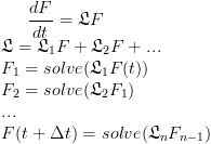
One interesting way you can solve PDEs is called "operator splitting". Basically, if the right hand side of our PDE is the sum of different components, we can solve those components separately in succession using different methods. This way if one part of the equation is stable with one method and another part is stable a different method, we can simply use which ever method is stable for each part. In operator notation we write:
This leads to so-called semi-implicit or implicit-explicit methods, where you use an implicit method for one part (diffusion) and an explicit method for another (reaction).
Multi-grid
One of the most efficient way of solving many PDEs including the diffusion equation is called the multigrid method. I will not go into the details here, but the idea is to iteratively solve the equation on grids of different "coarseness", which is increasing . It adds much additional complexity to the algorithm as you must switch between different grid sizes; however, it is a common method when speed is necessary.
Examples
Reaction Diffusion systems

2 part

Turing
ReactionA = rate*(a*b-a-alpha)
ReactionB = rate*(beta-a*b)

alpha = 8 to 20
beta = 8 to 20
diffusionA = ~1/16
diffusionB = ~1/4 - 1
rate = ~1/128 - 1/64
a_initial = ~4.0
b_initial = ~4.0
deltaT = .5-1

Gray Scott
ReactionA = rate*(a^2*b-(F+k)*a)
ReactionB = rate*(-a^2*b+F*(1-b))

k = ~.05-.06
F = ~.012-.04
diffusionA = .2
diffusionB = .1
a_initial = 1 with center ~.5
b_initial = 0 with center ~.25

complex patterns in a simple system

Brusselator
ReactionA = rate*(alpha-(1+beta)*a+a^2*b)
ReactionB = rate*(beta*a-a^2*b)

alpha = ~3
beta = ~9
rate = .5 to 2
diffusionA = 12.6/47.5 - 16.7/49.4
diffusionB = 27.5/141.5 - 36.4/117.6
a_initial = ~3.0
b_initial = ~3.0

[16] display of vector fields using a reaction diffusion model

Gierer-Meinhardt
ReactionA = rate*(gamma+a^2/b-alpha*a)
ReactionB = rate*(a^2-beta*b)

alpha ~ beta ~ .001-.005
gamma ~ 10^-4
Db > Da

[6] A theory of biological pattern formation
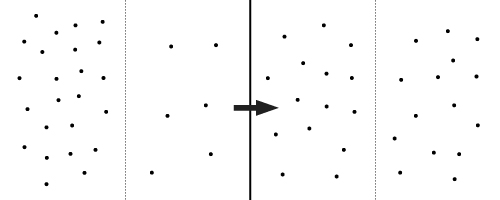 Diffusion is a passive spreading or averaging process. We think of it when we place a drop of dye in water or heat evens out in a room. More rigorously we can describe it as the motion en masse of particles moving randomly in a fluid. Here randomly means that the movement of a particle is independent of its previous state at any point in time, unlike Newtonian particles whose movement is dominated by forces and inertia. We are not concerned about the movement of an individual particle, but the aggregate motion of all the particles.
It is generally difficult to think about or describe random motion, but statistical mechanics gives us a partial differential equation which describes the evolution of the concentration of particles in space.
Diffusion is a passive spreading or averaging process. We think of it when we place a drop of dye in water or heat evens out in a room. More rigorously we can describe it as the motion en masse of particles moving randomly in a fluid. Here randomly means that the movement of a particle is independent of its previous state at any point in time, unlike Newtonian particles whose movement is dominated by forces and inertia. We are not concerned about the movement of an individual particle, but the aggregate motion of all the particles.
It is generally difficult to think about or describe random motion, but statistical mechanics gives us a partial differential equation which describes the evolution of the concentration of particles in space.


 A prototypical engineering problem is to find the temperature of some element given the heating conditions. This amounts to solving the heat equation which looks exactly like the diffusion equation. This leads us to the problem of boundary conditions. For instance, in one dimension we want to know what the temperature of a bar is if we are keeping one side at a constant temperature and the other side is cooling at a constant rate. Or how fast does it heat up if one side is insulated. We have to figure out how to define these conditions mathematically and then how to implement them in our simulation. In more than one dimension, we can start to make more complex boundary conditions that are non-rectilinear or change in space and time.
 and move forward in time with time steps of
  . We can employ several different difference approximations and integration methods to solve the PDE.

 is greater than .25, it will blow up. This limits the speed of the simulation since your time step will always have to be small. The error is also the same as the forward Euler method for ODEs.