Fluids are one of the most classic and difficult problems in modeling and simulation. Fluids also govern many interesting phenomena, almost anything involving the flow of air or water. Often of particular interest is the simulation of turbulence or chaotic flows. Because of the ubiquity and difficulty of the problem, almost every technique in physical simulation has been brought to bear. Here we will be discussing one method called smoothed particle hydrodynamics (SPH). This uses a particle system-esque formulation to represent continuous problems. The implementation of it is fairly simple, but conceptually it is somewhat complex. Keep that in mind as we discuss it.

There will be a lot of math here that may be conceptually difficult. The important thing is to focus on the ideas and not get lost in the equations. The generally accepted way of representing fluids is by a set of PDEs called the Navier-Stokes equations. Though they may appear as gibberish at first, these equations actually form an elegant description and are based on simple laws of conservation (momentum, energy, and mass). In general, we are interested in incompressible fluids. This means fluids whose density does not change. In most cases this is a correct assumption, but certain phenomena, like the propogation of sound or shock waves depend on compressions. Without going into detail on their derivation, here are the Navier-Stokes equations for an Newtonian incompressible fluid.


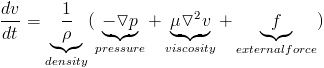
Now we can digest this equation a little bit. Note this gives us an equations for the change in velocity. We would have to integrate again to get position. External forces are simple, they are just like forces in point based physics such as gravity. Density here is acting like mass in a discrete system. So ignoring pressure and viscosity, this looks just like Newton's equation of motion.

The pressure term simply says that fluids move from higher to lower pressure. In more formal language it accounts for the normal stress. That is pretty straight forward, only where does the pressure come from. How do we compute it? If a fluid is truly incompressible and conditions like temperature are homogeneous, then the pressure is constant. Therefore, the gradient of the pressure is zero. However, in other circumstances we can use a so-called "equation of state" to determine pressure. These are equations like the ideal gas law.

In this case we use something similar.

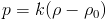
Where n/V is proportional to density and we simply lump the other terms into k. This equation says that pressure wants to equalize around some rest density, . k is a constant determining the speed with which it equalizes. By using the gradient of the pressure as a force, we are moving towards that rest density. Note that this tries to approximate an incompressible fluid. If k is very large, particles must stay at the rest density making it incompressible. This is only roughly based on physical intuition, and not on actual physical laws. Applications that require a more precise result might require a more realistic equation of state.

The viscosity term, , results from a simplification due to incompressibility. One aspect of this term that is confusing is that the laplacian usually applies to scalar fields, not vectors like velocity. In this case it refers to a vector made of the laplacian of each direction separately (in cartesian coordinates). This term says that velocities tend to average out or want to be the same.

One thing to note is how similar this is to the flocking simulation with multi-agent systems. The alignment rule is much like the viscosity. The pressure acts as the separation rule. The only thing absent is the cohesion rule, but that could be simulated as an attractive force between the particles. I just mention this to bring up the parallels between different phenomena and different simulation techniques. In fact real flocks have been observed to have fluid like properties like surface tension.

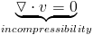
In this implementation of SPH we are ignoring the incompressibility equation. This equation states that divergence of the velocity is zero. Divergence measure how much of a source or sink a point in the field is, or put another way it measures how much an infinitesimal volume would stretch or shrink. So the divergence being zero everywhere says that no volume stretches or shrinks in the flow, thus the field done not compress. Solving this equation involves "projecting" the velocity field into a divergence free space. This can be a complex process, so here we merely approximate incompressibility.

One aspect that is missing from this definition of the Navier-Stokes equation which you often see is convection. This is often the most difficult part to deal with in many simulations and it comes from this equations.

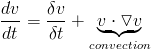
The convection term indicates that velocity is changing in space as well as time. In simulations with fixed points, you need to account for the flow or convection of the velocity. Our simulation will be based on moving particles, so this term is taken care of implicitly. This is convenient because one of the reasons the convection term is difficult to deal with is it is "non-linear" which means the velocity appears twice in the equation.

Smoothed particle hydrodynamics was originally developed for astrophysics simulations, but has been applied to various continuous domains such as fluids and elastic solids. It is the technique used by most commercial computer animation softwares to simulate fluids. The idea behind smoothed particle hydrodynamics is that continuous quantities are represented by discrete particles that have some area of influence. Instead of being point masses they are fuzzy quantities that fade with distance.

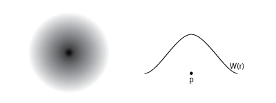
This is accomplished using a kernel or smoothing function, W(r), which drops off with distance from a particle. Each particle holds various properties like density, velocity, perhaps temperature or other custom quantities. To find these quantities at any point in space separate from the particles you simply sum them all up with the weights.
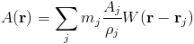
This is the equation to compute some quantity, A, defined on each particle at any point in space, where r indicates position and we are summing over all particles. We are normalizing by volume (or mass over density) because each quantity of the particle is actually spread over some volume. What makes this method nice is how we can then estimate differentials. Recall that in the finite difference method we used subtraction between neighboring values to estimate differentials, and there were many different methods for doing so. Here we can simply apply differential precisely.

Because the quantites at the particles are actually constants, the differential only applies to the kernel function. Since we choose the kernel function, we can also get an analytical equation for its derivative. This allows us to easily calculate any derivative. Now solving our differential equation is fairly straight forward.

First I want to mention some terminology used to classify different methods for solving PDEs. The simplest is mesh versus meshless. SPH is a meshless method. There is no underlying structure to the simulation, and the relationship between different points is completely dynamic. This allows greater flexibility and simplicity. Mesh methods can be further divided into grid and more general mesh methods. Grid methods work on a regular grid, all the cells of the grid are identical. The finite difference methods we used to model diffusion fall under this category. They are very simple, but have difficulties conforming to less homogeneous conditions. Finite element methods, which we have not discussed, generally work on arbitrary triangular meshes.

A more pneuonced distinction is Lagragian versus Eulerian methods. Eulerian methods look at quantities in at a fixed point in space. For instance finite difference methods are Eulerian. In these methods the convection term of the Navier-Stokes equation is very important. Lagragian methods follow quantities as they move, so SPH is Lagragian. Here convection is handled implicitly because the particle positions are moved as you integrate. Lagragian methods are useful when talking about moving objects such as deformable bodies.

We can now solve the Navier-Stokes equation in much the same way as we solved point mass particle systems. The only addition is we have to solve the pressure and viscosity forces along with any external forces. We can then use any integrator (Forward Euler or RK4) to compute the new position and velocity.

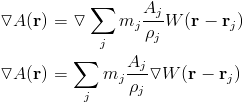
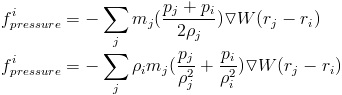
First the pressure force. We compute the force the same way as we computed density. For each particle, the force is computed at that particles position.

There is a subtle problem with this equation. It leads to asymmetric forces. As we know, every action must have an equal and opposite reaction. Two approaches to making it symmetric have been suggested. They involve mathematically intuitive, but physically dubious revisions.

Now we have to compute the pressure at each point, which we can do based off our equation of state.

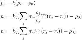
Note the bit of trickery to get an expression for computing density at each point. In computation, we would do this in several steps. First we compute the density at each particle. We use that to determine the pressure at each particle. Then we use the pressure at each particle to compute the pressure force.

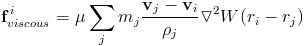
The last remaining piece is viscosity.

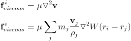
Here this is also asymmetric. The way it is symmetrized it is by looking at the relative velocity between the two particles. This makes sense intuitively in that there is no viscous force if all the particles are moving at the same velocity.

The one unaddressed portion of this whole discussion is the kernel function. What is it and where does it come from? The kernel function really defines the way all these forces act, so it is very important to smoothed particle hydrodynamics. There are a few properties that all kernel functions must have. They must be symmetric as in they are equivalent no matter what side you are on:

They all must be normalized, as in they must sum to one. If a quantity is spread over some volume, then if you add up that quantity weighted by your kernel function in all space, you want to get the same quantity back.
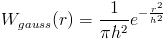
The kernels have to go to zero at some specified smoothing distance, h. In addition, we want the derivatives also to go to zero at the same distance. The original formulation of SPH used a Gaussian function as the ideal kernel. This is your typical bell curve. However, it is computationally expensive, so other kernels have been developed that are based on polynomial splines.


In our model, for stability and accuracy we end up choosing different kernels for different purposes. Essentially we want each derivative of the kernel to have different properties, so we design a different kernel for the pressure gradient and the viscous force laplacian.

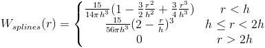
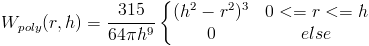
For the undifferentiated kernel, which we use to calculate density, we want a kernel that looks like a gaussian curve, a nice even distrobution. We also want it to be easy to compute. A suggested function is:

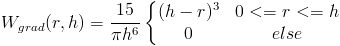
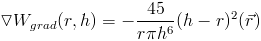
Problems occur for this kernel when we look at the gradient. The gradient determines the pressure force, and in this function the gradient tends towards zero as distance tends towards zero. This means the pressure gets weaker when particles get closer. This is exactly the opposite effect we want. So we can design a kernel for pressure in which we only care about the gradient.


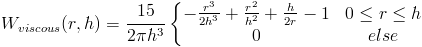
Both of these kernels have the property that the laplacian is sometimes negative. However, we never want a negative viscous force. Therefore we need a kernel function whose laplacian is always positive.


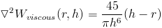
So we use the first kernel when talking about undifferentiated quantities, the second for the gradient, and the third for the laplacian.

As with many systems, choosing the right parameters is both essential and difficult. Here we both look to physical reality for guidance, but also consider the numerical stability of our simulation.

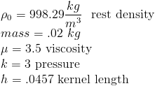
The density, mass and kernel length are realistic for water. However, the pressure constant is tiny compared to one computed using the ideal gas law. This should be as high as possible while still maintaining stability. Also, the viscosity is much higher than in reality. The kernel radius should be as small as possible, to reduce the amount of computation, but must include enough neighboring particles to allow for realistic behavior. These are just example values, and others are certainly possible.

You will note that there are a lot of somewhat seemingly adhoc adjustments and estimations to get SPH to work. We make changes to have forces so they make more physical sense. We assume incompressibility in our equations without actually enforcing incompressibility. We also have the weird fuzzy particles, which do not have much of a physical justification. So while SPH is a simple, flexible way of simulating fluids, it does have its problems. We will go over the steps of an basic SPH simulation.

1. Compute density and pressurefor all particles
2. Compute pressure and viscous forces for all particles
3. Compute any external forces (like gravity)
4. Sum all forces
5. Integrate position and velocity with any old integrator (Leapfrog is common)
6. repeat

How do we visualize the fluid? We can interpret this fluid representation as an implicit surface or a level set. There are many methods for drawing such surfaces. One of which we have encountered before is marching cubes. We can also visualize the fluids with what are called "tracer particles". These are imaginary particles whose position we follow as it flows through the velocity field. They are often used for smoke-like effects.

How do we deal with boundary conditions? One method is pretending there are particles along boundaries, and the pressure force pushes back on the fluid. This method can be unrealistic. More complex methods involve actually enforcing incompressibility using Poisson solvers, which remove any velocity component normal to the boundary.

We may want to add additional properties to our fluid. One common property required for realistic fluids is surface tension. We can also look into multiple fluid interactions. Friction may be required at boundary conditions.

How can we extend SPH? We can look at other continuous problems with SPH. A common one is looking at elastic stress in solids. Can it make any sense to use SPH to solve reaction diffusion problems in which particles would not move? We can also add more elements to our fluid model like temperature or transport models for erosion and deposition.

We will address some of these issues in the following class.