The basic SPH model can be improved, extended and reused in many different ways. Though it was developed for astrophysics it has been applied to almost every common problem that can be framed as a PDE. Along the way different elements have been added to the model. Here we will discuss a few different ways to use SPH.

• Surface tension
• Buoyancy
• Boundaries
• Visualization
  • Tracer particles
  • Marching cubes
  • Point splatting
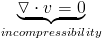
• Incompressibility
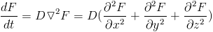
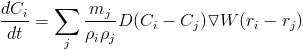
• Diffusion

Surface tension is caused by the cohesion of fluid particles, and it is not included in the Navier-Stokes description, which is only based on conservation laws. However, surface tension is necessary for realistic fluid motion. Surface tension occurs only on the "free surface" of the liquid where the cohesive forces of the liquid are asymmetric. There have been a few different approaches to modeling surface tension in SPH. We look at two: one which looks at the curvature of the surface of the fluid, and one which attempts to directly model cohesive force.

To define the surface of the fluid, we use a so called "color function", defines the shape of our fluid.

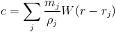
We can interpret this as the weighted "volume" from each particle. Using this, we define the normal of our surface as the gradient of the color field. The direction in which color is most increasing points inward toward the surface. Here we use the standard kernel, not one modified for specific behavior in the gradient or laplacian.

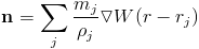
Surface particles are identified as particles whose normal length excedes a certain threshold. The surface tension force is only evaluated at these points.

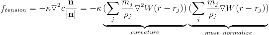
Surface tension wants to minimize curvature. This is why droplets tend to form spheres (in the absense of gravity). The curvature of our surface can be estimated as the laplacian of the color field. So our surface tension force is normal to the surface and proportional to the curvature. The force is also scaled by some surface tension strength, K.

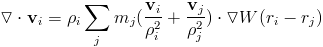
Another approach creates an articial attractive force, and does not calculate the surface of the fluid. This approach is used because the laplacian calculation can be error prone especially in areas with sparse particles. The force is a very simple attraction weighted by the kernel function. Note that this equation is a direct modification of the acceleration, not the force.

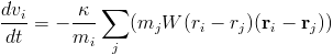
Another thing to note is that this method reuses the kernel functions used to calculate the density. Instead of recalculating them, we can simply store them for later use. This method is from Becker.

For gaseous fluids we may want to implement a buoyant force such as when a plume of smoke rises. In reality this is caused by temperature differences. So one way to add this to our model would be to add temperature. Temperature effects the rest density of the fluid and the pressure force. It also has the added property that it diffuses. One way to fake this buoyancy is to create an artificial buoyant force. This can be used in place of gravity.

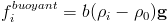
Where b is an artificial buoyancy strength.

In order to have a fluid simulation, we need to have boundaries, unless our fluid is simply floating in space (not very interesting). This could be as simple as a containing cube or as complex as terrain with moving boundary objects. There are multiple ways to implement boundaries, such that the fluid does not penetrate into them.

One method is to take a collision handling approach. We treat a particle penetrating a boundary surface as a collision. Collision handling is an entire topic in and of itself, but we will discuss some options briefly. The first task is collision detection, or finding out when a particle has penetrated a boundary. For simple shapes this is easy. For instance, in a cube that is oriented with the coordinate axes, we only have to test if the particle is within a certain range in each coordinate. Or if we have a implicit equation for our surface, we can simply evaluate that equation for our particle. For complex shapes represented by triangular or tetrahedral meshes this process becomes much more complex. First, checking each triangle for each particle would be a very computationally intensive process, so we need to come up with methods to speed up this process. Additionally, if the triangles/tetrahedrons are small enough, a particle might pass through multiple ones in a single step.

Once a collision is detected, we have to correct it. The simplest method is projection. Simply move the particle to the closest point on the surface. One again for a cube or an implicit surface, this is easy mathematical operation. We also want to correct the particle's velocity. If a particle has hit a boundary we want to the particle to stop moving towards this boundary. It may also bounce off the boundary. This is done by modifying the portion of velocity that is normal to the boundary surface.

Where c is a coefficient of restitution which determines how bouncy the collision is.

A slightly more accurate and complex way to handle collisions is to find the exact time and position of the collision. This means going backward in time until the point of intersection. We move the particle to the intersection point and correct the velocity by the normal at that point. We then take a partial integration step forward using the corrected velocity with a time step that is rest of the time step after the time of intersection.

In short collision methods are easy to implement and efficient for simple shapes, but for complex shapes they become difficult. They also treat the fluid as point particles and do not take into account their continuum nature. A good write up of this method can be found in Kelager, section 4.

An easy to implement but generally unsatifactory method is to use penalty forces. This method adds a force pushing away from the surface in the case of a penetration. Often, the force is a spring-like and gets stronger the deeper the penetration. This can lead to unrealistic behavior, and some minimal penetration. However, it is simple to implement because it fits into the existing force framework of the simulation. The force can look like:

Where d is the penetration depth, K is a penalty strength, D is a dampening coefficient.

A more common method for boundaries in SPH is using fictitious boundary particles. We place particles with a regular density on the surface and insert them into our regular fluid solving framework. We can use the pressure force caused by these particles to push against any fluid particles that want to penetrate the surface. One thing to note about the method is that pressure force is caused by a pressure gradient. Therefore, the pressure (or density) of the boundary must be greater than the fluid in order to push back. This could be changed dynamically based on the density of the fluid it is pushing against. Additionally, for an accurate pressure force it is beneficial to have multiple layers of particles (based on the kernel radius) on the boundary.

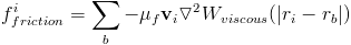
Another property that a boundary can have is a so-called "no slip" condition. This basically means that the surface applies some friction to the fluid. This is implemented using the viscosity force, with the velocity of the boundary being zero. Instead of the viscosity constant, we use a different friction constant in our calculation.

There are many ways to render a fluid. The simplest which we have already seen is drawing spheres for each particle. Obviously this is very unsatisfactory. We need other ways to visualize a fluid that look more realistic.

One of the simplest ways, which is often used for gaseous effects is using tracer particles. These are particles that move through the fluid. We initialize the particles in some, slightly randomized location, and allow the particles to advected through the fluid drawing their path. This involves computing the velocity at each point using the SPH particles and kernels, and moving them through euler integration. The particles do not need velocity themselves, since they are only used to visualize the motion of the fluid. This works well for effects like smoke or other ethereal substances, but does not convey a solid fluid like water.

There are two primary ways to visualize the fluid surface. Both are based on the color function we defined earlier. One uses implicit surfaces. These are surfaces defined by what volumes are enclosed by the surface, not by the boundary of the surface. We use the color function as our implicit surface. We then set some threshold value which we say defines the boundary of our surface. All points less then that value are outside, and all points greater than that value are inside. There are then multiple algorithms for extracting a mesh from this function. The simplest and fastest is called marching cubes. This method discretizes the implicit function by evaluating it at regular points on a grid. For each cell of the grid, we define whether each corner is inside or outside the surface. Then we map each of the 256 possible configuration to a surface that goes in that cell. We do this for each cell in the grid. To speed up the process use the normal from the color function to determine the SPH particles which are on the boundary of the surface. We only perform the marching cubes algorithm around these points. This marching cubes version evaluates the surface at every point. This uses a lot of computation and memory. A smarter algorithm would use a HashMap to store values and only evaluate points that we know are near the surface, based on proximity to particles with a certain color value.

Obviously, there are inherent limits of the smoothness, accuracy, and resolution of this method. More complex methods involve mesh refinement techniques where you can specify how accurate you need your surface to be. These are significantly more computationally expensive, but if you only need to get the surface once (say for cnc production) they will provide a much nicer surface.

Actually creating a mesh is computationally intensive even using marching cubes. So for doing real-time rendering other techniques have been developed that do not actually involve defining a specific surface. These are point based rendering methods. A common one is called surface point splatting. This method involves drawing a circle (or other shape) for each particle that is on the surface. The circle is oriented toward the normal of the surface. Each circle is drawn such that its values (color, normals, etc) blend with neighboring circles. This requires somewhat complex rendering techniques often using advanced functions in opengl. We want to define a texture for each circle which contains the color and normals of the surface and which dissipates with distance. Then we blend the values of overlapping circles to get a smooth appearance. A simple version can be done directly in Processing without direct OpenGL manipulation simply by drawing the circles without blending.

Enforcing incompressibility through the pressure force both leads to very unstable simulations (necessitating a small time step) and overly damped fluid behavior. Instead of truly turbulent behavior, things tend to average out. In many other fluid simulations, incompressibility is handled through another means, called projection. These methods attempt to directly solve the incompressibility condition. In practice, these methods use a different computation of pressure to enforce incompressibility.

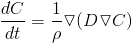
As it so happens, every vector field can be decomposed into two parts, a divergence free part and the gradient of a scalar field (which is curl free).

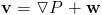
Where w is divergence free.

We can solve for the gradient component by taking the divergence of both sides. The divergence of the divergence free part is clearly zero, so it disappears leaving us with a Poisson equation, laplacian on one side and the divergence of the current velocity field on the other. We have seen Poisson equations arise when solving diffusion as well, when using implicit integrators.

We solve this equation for P, and then subtract the gradient of P from the current velocity, just as if we computed the pressure using density instead. The question in this case becomes how to properly represent the laplacian of the pressure and the divergence of the velocity. There are several different ways of doing so. The primarly issue is what occurs at boundary conditions.

One way to compute the divergence of the velocity is using the following formula.

We can come up with an equation for the laplacian of the pressure using the following equation.

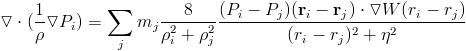
The equations can be solved using a standard sparse matrix solver like conjugate gradient. A sparse matrix library with several implemented solvers can be found here. The trick is what to do at boundary conditions. This method suggests using imaginary particles reflected over boundaries. It has also been proposed to simply use boundary particles. For more information on this method see Cummins and Rudman.

Another method described in Sin, et al. sets up the Poisson equation using a finite volume method. The volumes are created by taking the voronoi diagram of the particles and cropping by the boundaries. This is a clean way of dealing with boundary conditions, but computing the voronoi diagram can be a difficult (in computation and implementation) task.

Fluids often carry substances which diffuse. Temperature is the most common quantity which fluids carry and which also diffuses, but you may also model sediment or chemical transportation. As we have seen the diffusion equation looks like this.

Here we will look at a slightly different form.

Instead of using the laplacian of the kernel, we use an estimate of the laplacian combining the difference between the concentration at each point and the gradient of the kernel. This is called an integral approximation of the second derivative. This leads to more stable results than simply using the laplacian. For the diffusion rate, something around 0.1, might be a good value.

The diffusion equation can then be solved using either explicit methods or implicit ones as we did in with finite difference. We can use this method to model systems with advection and diffusion such as advection reaction diffusion or sediment transportation models.