Meet the Flummoxagon

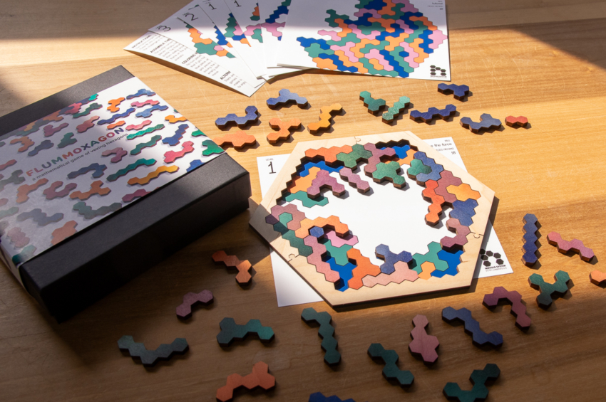
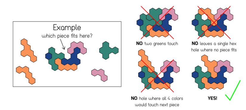
We’re excited to announce Flummoxagon, a new geometric puzzle game that might just leave you flummoxed. Imagine a mash-up of Pentominoes and Sudoku. Your goal is to fit all the pieces into the hexagon frame but there’s a twist, pieces of the same color can’t touch.  

It’s a fiendishly fun mix of Tetris-style block packing and logic-based constraint solving. The game ships with 13 gameboards, featuring puzzles from beginner to advanced, and new boards are added weekly to our website.

You can buy Flummoxagon now in our shop for $45. For the first month, take 20% off with the coupon code FLUMMOX (ends 10/31/2025).

How do you play?

Flummoxagon is made up of 48 tiles representing every shape you can make by joining up to 5 hexagons. All the tiles fit into a hexagonal frame and they come in 4 colors. There are 12 pieces of each color and 54 hexagons of each color (except green since there are an odd number of hexagons in the grid). The challenge is to place every piece into the frame without letting two tiles of the same color touch.  Now, there are hundreds of thousands of ways to do this; however, finding one on your own is nearly impossible (though let us know if you manage it!). 

Instead of an empty grid, to play the Flummoxagon, you start with a partially filled gameboard that only has one unique solution, just like a Sudoku. Each gameboard creates a challenging puzzle to solve. The puzzle ships with 13 of these gameboards of varying levels of difficulty, and we add new puzzles weekly on our website for endless challenges.

How did we get here?

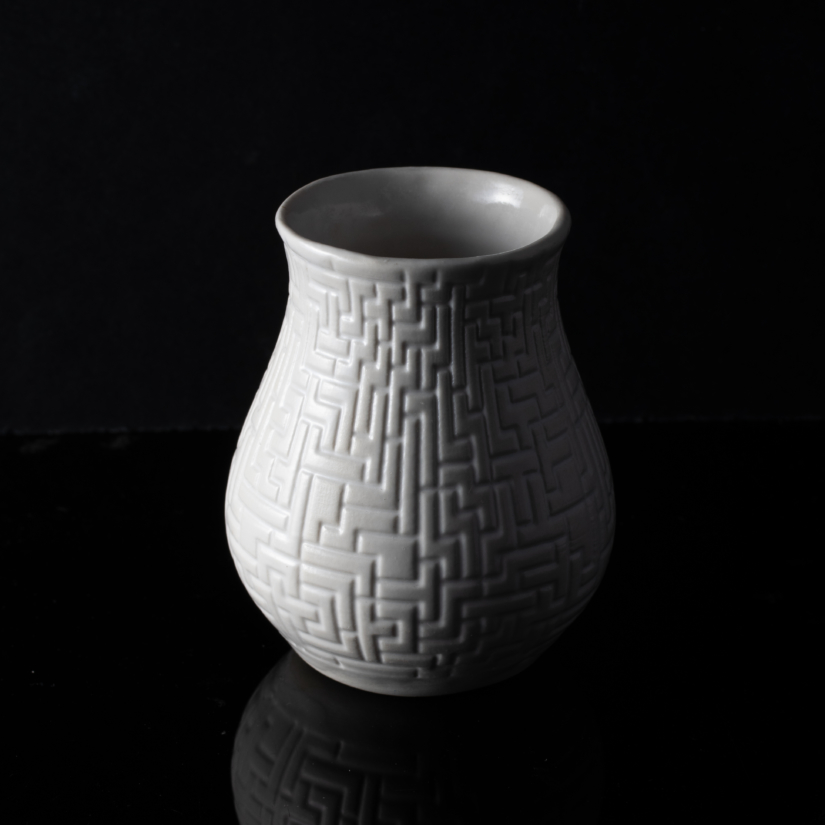
Jules has been interested in these kinds of tiling patterns since before he worked at Nervous System. He built a solver for placing tiles on a grid which is a version of a problem called an “exact cover.” Instead of a puzzle, he used it to make patterns which he turned into cast vessels. When he started working here, he wanted to use it to make a puzzle, which he did for friends and family. The first version had no colors. There were two problems turning this into a product. First, it already exists. Other people have made polyhex puzzles before. Second, more interestingly, was the playability. It took him 20-30 minutes to solve the puzzle. Even though the puzzle has millions of solutions without colors, there’s not really much of a reason to find another one. That gave us the idea to add a coloring to the pieces. This gives you a way to meaningfully differentiate solutions. You could ignore colors, you could say all like colors need to touch, or (like the classic map coloring problem) that no two alike colors could touch. That gives you a reason to put it together multiple times.

However, we quickly realized that even though there are still hundreds of thousands of solutions to the puzzle with the coloring rule, actually finding one as a human is extremely difficult. Maybe someone could do it, but it would take a lot of luck, a lot of time, or both. So it doesn’t add a lot of playability if one of the ways you can do it is essentially impossible (unless you’re a masochist). This led us to the insight that really makes this puzzle fun. What if instead of doing the full colored puzzle, we find partial sets of tiles where there is only one unique solution? This adds enough constraints to the problem that it becomes feasible. Now we’ve created something that’s more like Sudoku than a tiling puzzle. Each scenario presents a new set of constraints to solve. And we have near endless possibilities for designing new puzzle scenarios that range from easy to extremely difficult. We didn’t just make 1 new way of putting together the puzzle, we made a whole new family of puzzles.

This also justified having an automatic solver, which is what we were actually excited about in the first place. The original version of the puzzle didn’t really need the solver at all. Sure, you could find thousands of solutions, but to what end? Now the solver is an integral ingredient in the puzzle. Not only do we use it to generate scenarios, we also use it to grade the difficulty of them (without having to do every one ourselves).

Technical Details

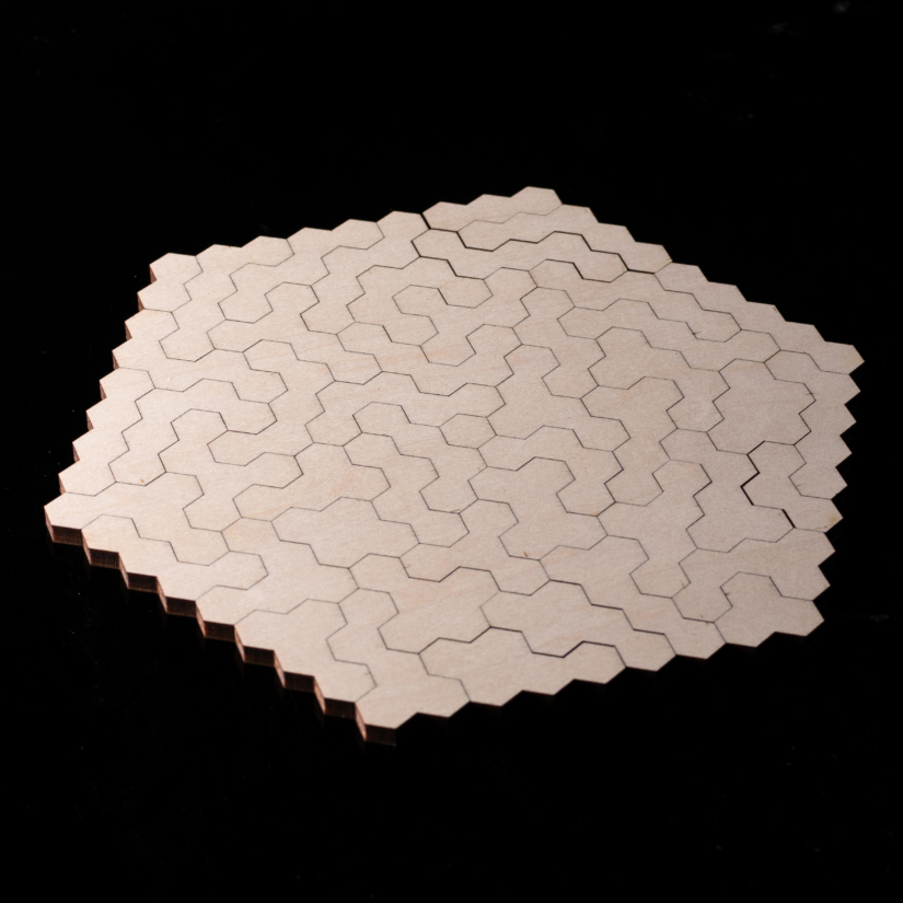
The tiling solver is really the crux of this project. The method is from the famous computer scientist Donald Knuth and involves a clever representation of the problem to enable efficiently searching for solutions. Consider the problem of placing the polyhex tiles of size one through three onto the pictured grid.

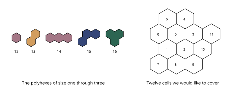
In exact cover, there is a universe of elements and a collection of subsets of those elements. The problem is to choose some of those subsets so that each element in the universe is represented exactly once. In the case of tile placement, there is one element for each cell in the grid to be covered, and one element for each tile’s name. Every valid tile placement is represented by a corresponding subset of these elements. If we number the grid and tiles as shown, we could represent placing the single hex tile in the upper left hex of the grid as {5,12} or placing the straight three tile hex along the bottom of the grid as {7,8,9,14}. We could then represent all possible tile placements as an array with columns identified to the grid cells and tile names and with one row for every possible tile placement.

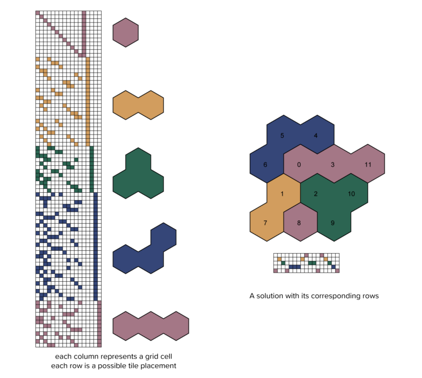
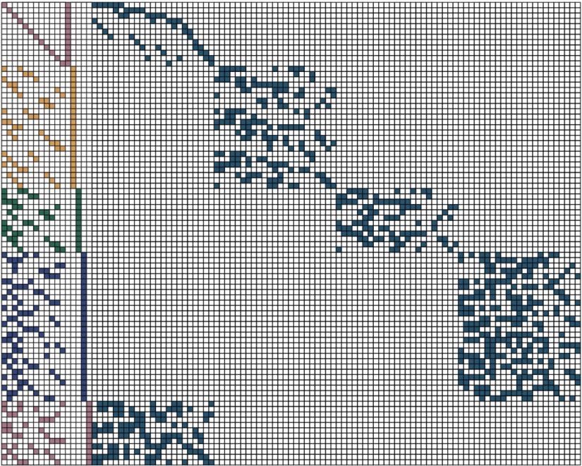
The columns of the above array represent constraints that must be fulfilled in every tiling of the grid; each cell must be covered by a single tile and each tile must be placed into the grid exactly once. In order to represent the constraint that no two tiles of the same color may touch, you can introduce “optional columns” representing a color touching an edge in the grid. For each edge in the grid, four columns are added to our array, one for each color. These columns are not required to be covered at all, but are required not to be covered more than once, as that would represent two tiles of the same color touching. 

Donald Knuth popularized a simple algorithm for solving this problem called Algorithm X. Algorithm X is based on the observation that each column can be considered sequentially when searching for a solution. Choose a column to cover, then choose a row that covers that column. Then look along the row you chose and delete every other row that shares a column with that row, since those rows can’t be part of a solution with the row you already chose. 

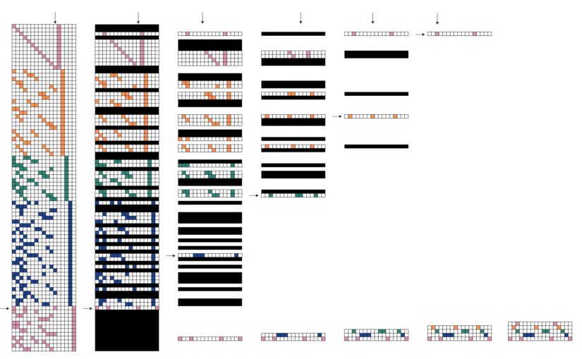
If the array has an empty column with no rows to fill it then you have to backtrack by adding all the rows you deleted in the last step back into the array and choosing another row. Then if there are no more rows to choose from in your chosen column you also need to backtrack. If all the columns are covered, then you have found a solution.  

The naïve approach of deleting and re-adding rows to an array has two problems: The first is that the arrays that show up in covering problems tend to be very sparse and so are expensive to store as solid blocks of zeroes and ones. The second is that repeatedly deleting and re-adding rows to an array is very time consuming.

Knuth introduced a technique called Dancing Links that makes this kind of search much more efficient. The idea hinges on the reversibility of deleting an element from a linked list. In a doubly linked list, each element points to its neighbors, and to travel along it either left or right you just follow the arrows from one element to the next. 

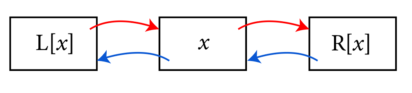
To delete x from the list, you need to make the neighbors of x point past x to each other. Importantly, this doesn’t change the things x itself is pointing to:

R[L[x]] = R[x] and L[R[x]] = L[x]

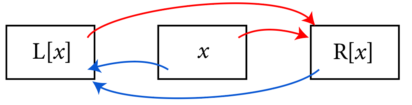
To put x back into the list, you can just say that the things x is pointing to should point back to it:

R[L[x]] = x and L[R[x]] = x

You can use this idea to represent the array as a linked structure where every element points to its four neighbors in row and column, and rather than erasing rows from the array you can “cover” and “uncover” them using these operations. This representation is much smaller in memory, and it avoids the problem of clearing and reallocating memory, making it much faster.