
Holiday Sale – 20% off
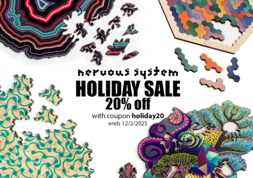
It’s time for our annual sale! Take 20% off most items with the code HOLIDAY20 (ends on Tuesday 12/2/2025). The coupon code must…
It’s time for our annual sale! Take 20% off most items with the code HOLIDAY20 (ends on Tuesday 12/2/2025). The coupon code must…
The Bismuth Crystal Puzzle is the successor to our popular Geode and Agate puzzles; the next in our growing line of unique geological…
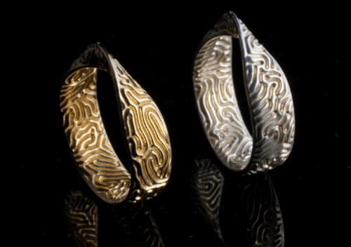
Someone asked us to make Reaction-diffusion wedding bands, we liked the resulting rings so much we decided to make an entire Reaction jewelry…
Explore endless fields of color and pattern with our Marbling Infinity Puzzle made in collaboration with artist Amanda Ghassaei. Intricate wooden puzzle pieces…
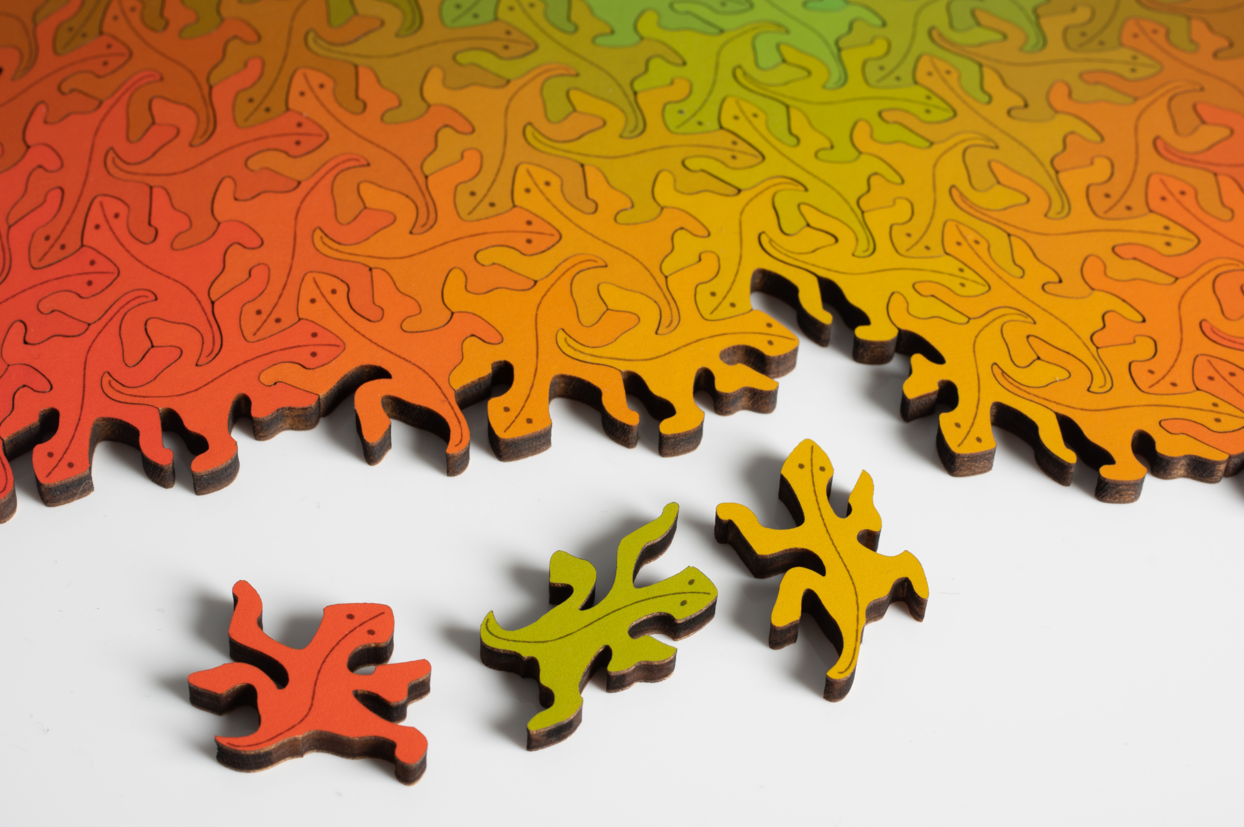
Have you ever done a puzzle that has no beginning or end? Can you tame the Lizard Infinity Puzzle™? Hundreds of unique lizards…
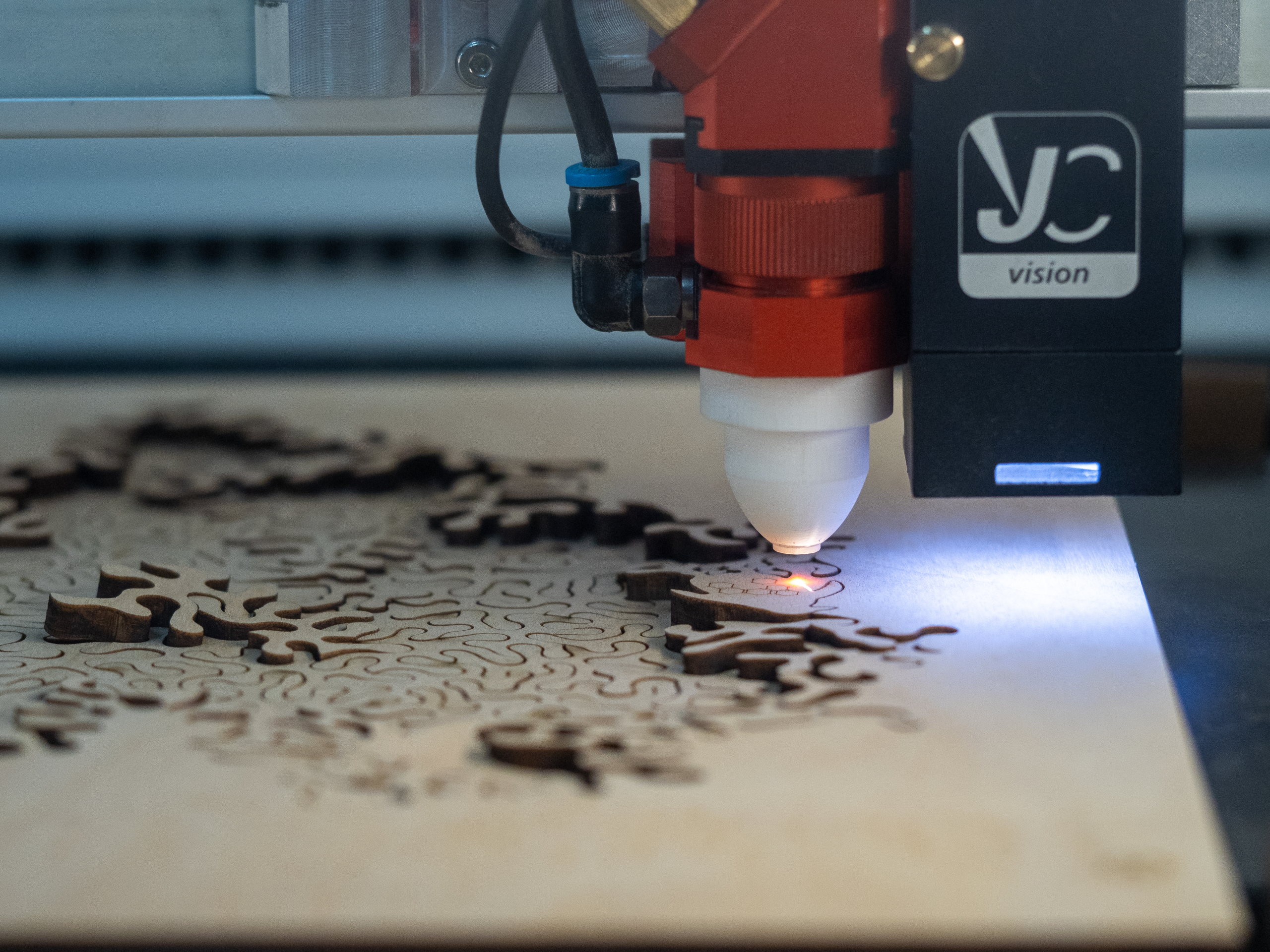
People often ask us for tips on how to make lasercut jigsaw puzzles. In fact, our most popular blog post is on our…
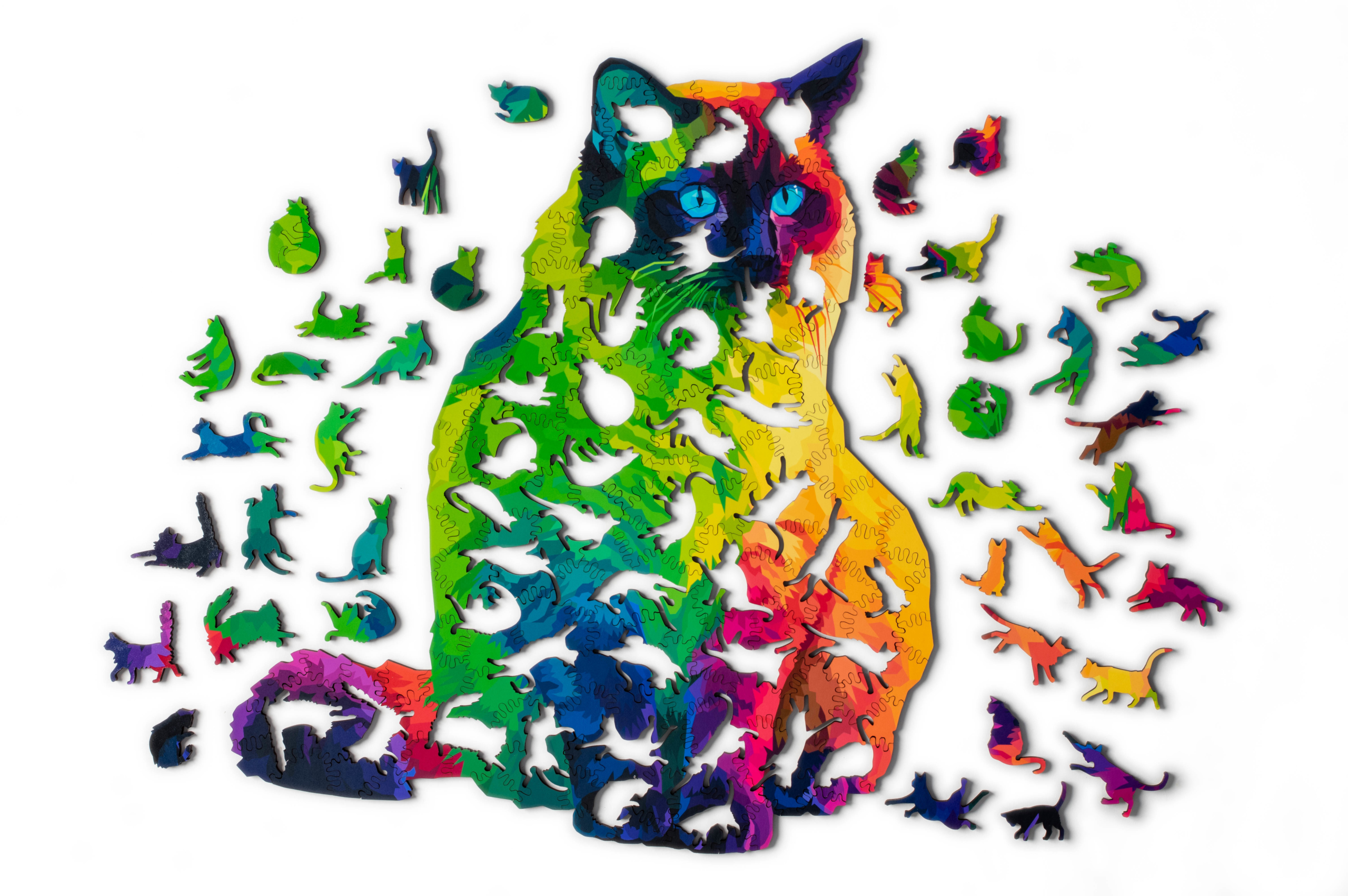
We’ve combined all of our prowess in computation and fabrication to bring you the ultimate cat jigsaw puzzle! Herding Cats is a technicolor cat…
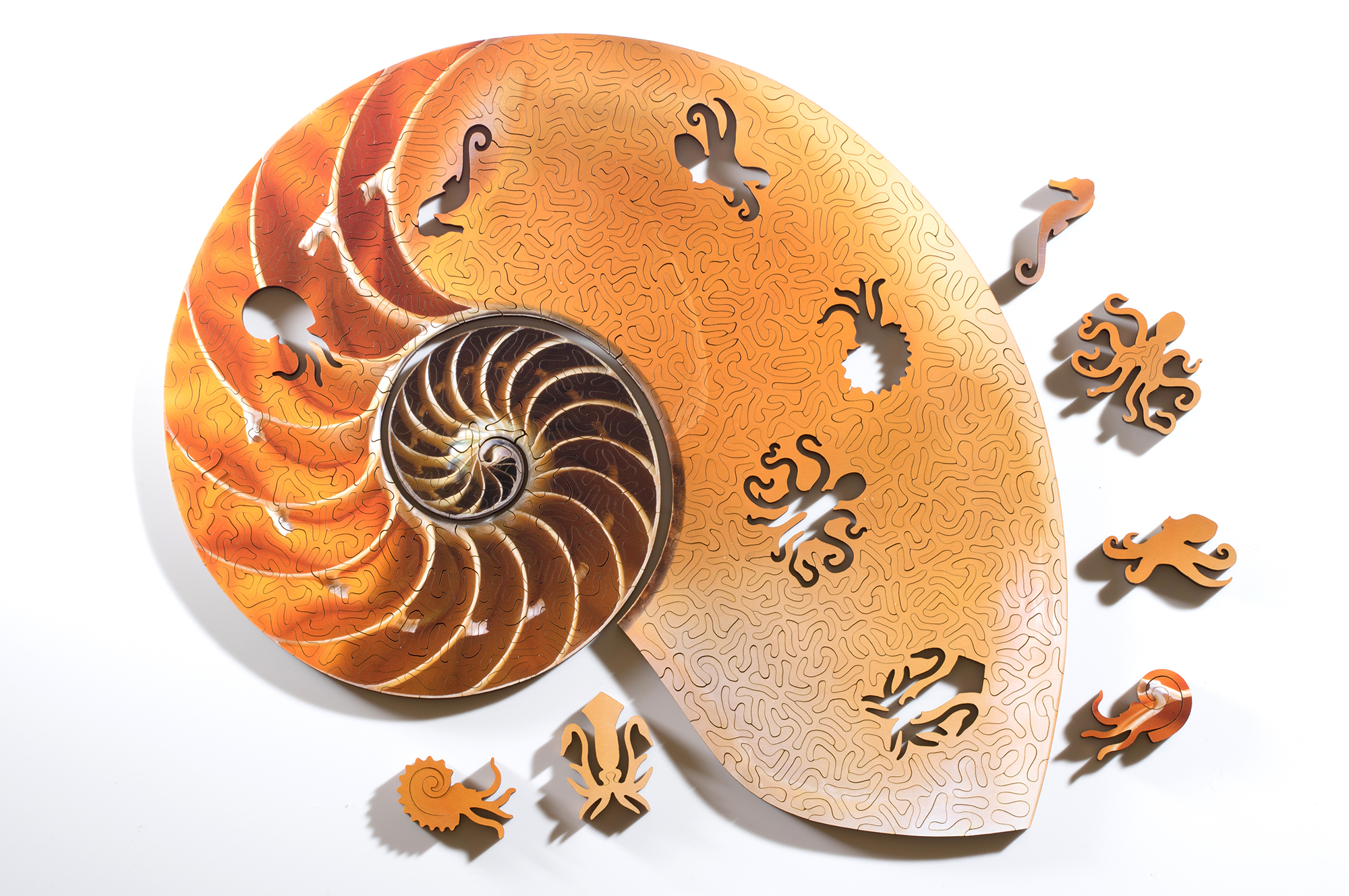
The Spiral Puzzle is a twist on traditional jigsaw puzzles. Usually you begin a puzzle by assembling the edge pieces and then work…

Nervous System Moves to the Catskills Big news! We are relocating from Somerville, MA, our home for the last 8 years, to the Catskills in New…
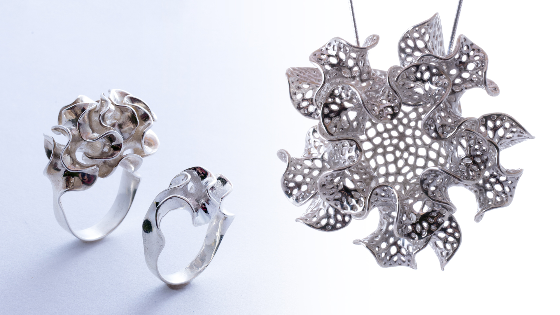
Introducing Floraform, the latest generative design system from Nervous System. Floraform is inspired by the biomechanics of growing leaves and blooming flowers and…