
Porifera – 3D printed ceramic jewelry
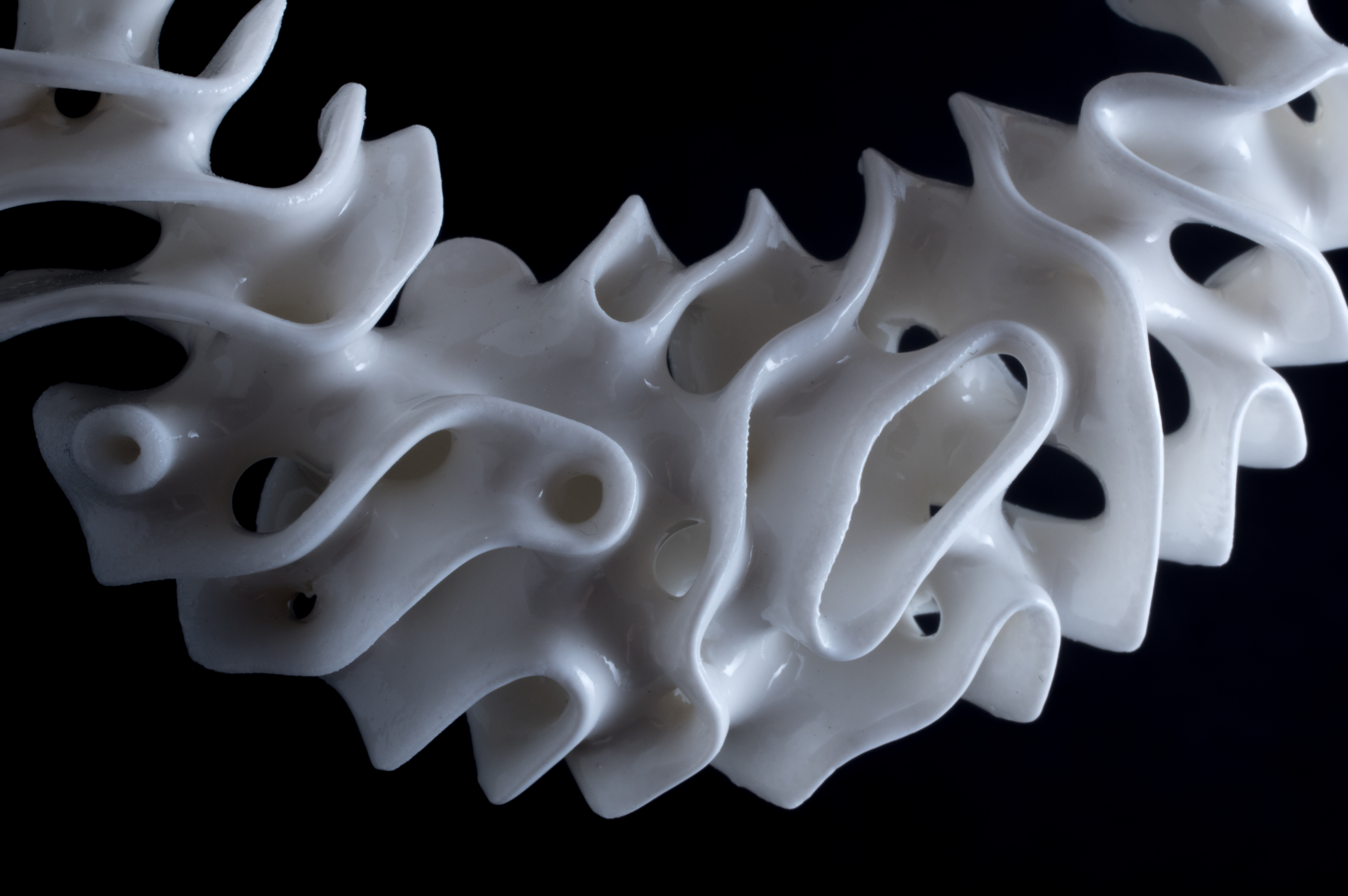
Porifera is a new jewelry collection by Nervous System inspired by the forms of deep-sea glass sponges and made in a new 3D-printed…
Porifera is a new jewelry collection by Nervous System inspired by the forms of deep-sea glass sponges and made in a new 3D-printed…
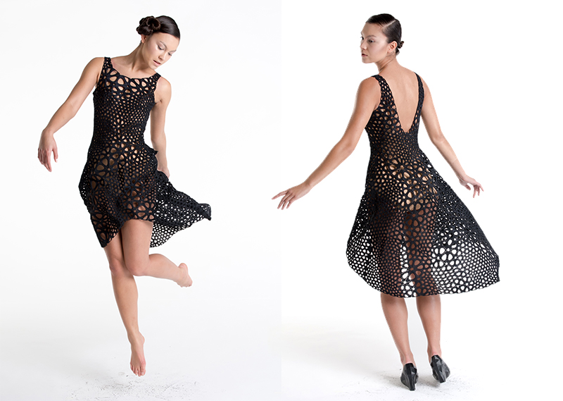
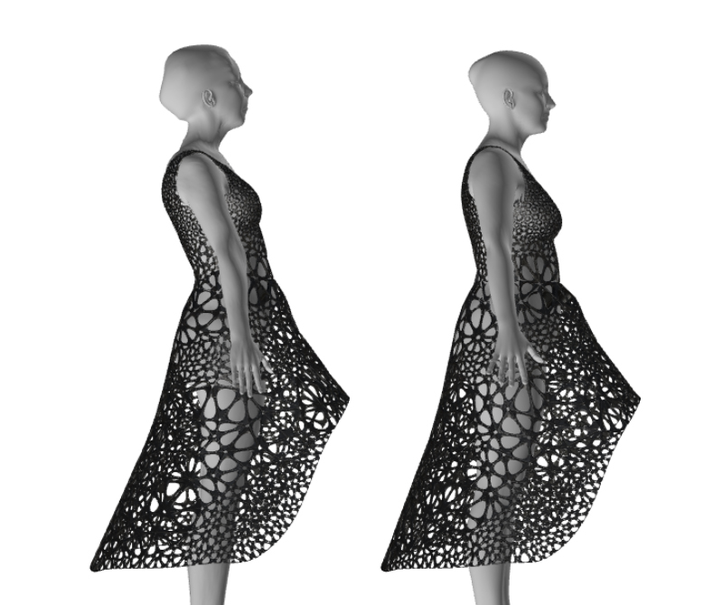
We have created the first dress with Kinematics, our 4D printing system for generating complex, foldable forms. The Museum of Modern Art has…
We’ve added something new to our lineup of customizable products: jigsaw puzzles! You can now make a plywood puzzle with your art in…
Finally, we have some progress to share on something we’ve been working on for a long time! This project focuses on the differential…
Nervous System is headed to San Francisco to exhibit at O’Reilly’s Solid, a new conference focusing on innovation at the intersection of hardware…
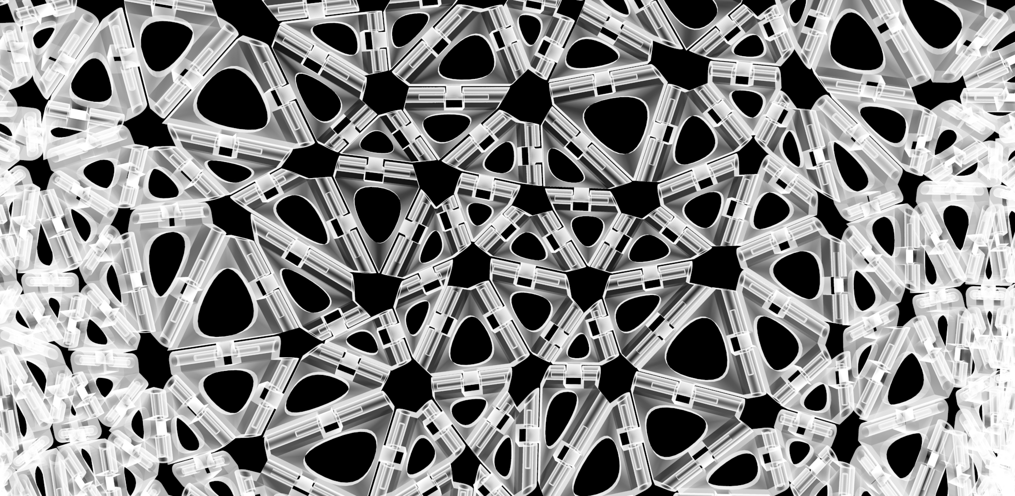
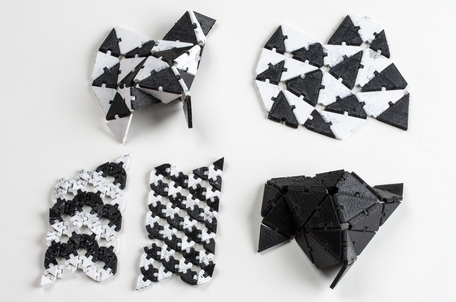
Kinematics is a system for 4D printing that creates complex, foldable forms composed of articulated modules. The system provides a way to turn…
Most of our projects start with a natural inspiration, but Kinematics emerged from a very different perspective. This project started with a technical…
In order to generate the price of a custom design on the fly, we need to calculate the volume of the piece for…
Folium is a generative jewelry series inspired by the algorithmic structures of plants and algae. Each Folium design is one of a kind,…
Recently, I came across a neat data structure called a pairing heap. Now, if you’re not familiar with the term heap it can sound…