
Xylem Arbor
We recently created our first large scale public artwork. Soaring to a height of 120′, Xylem Arbor is an aggregation of bent metal…
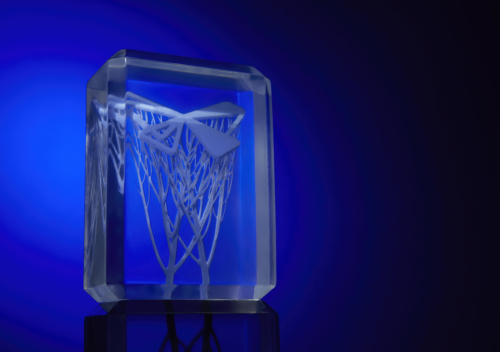
Nervous System’s design for Formlabs‘ 2022 Impact Award Trophy was informed by their work designing vascular networks for 3D-printed organs. Intricate branching fluidic networks printed…
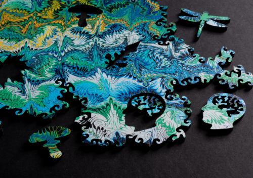
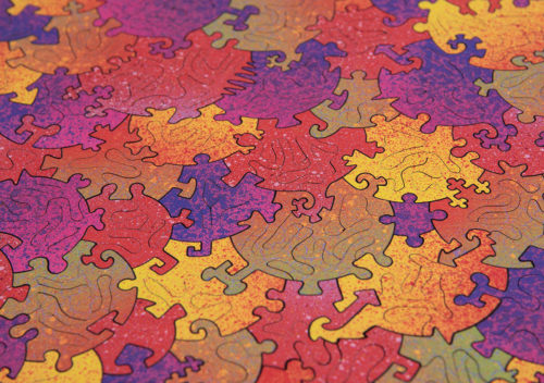
Explore endless fields of color and pattern with our Marbling Infinity Puzzle made in collaboration with artist Amanda Ghassaei. Intricate wooden puzzle pieces…
Yellow moon gyroid is a sculpture we created to honor the work of mathematician Alan Schoen. It is now permanently installed at the…
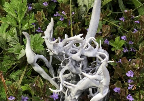
Hi, I’m Sage Jenson and I was recently artist-in-residence at Nervous System. As part of my work, I create GPU-based simulations inspired by natural phenomena, from slime mold to snow. Jesse, Jessica and the team at Nervous System helped me translate my digital simulations into physical objects through 3D-printing, metal casting and traditional 2D-printing. Creating these objects pushed the technical boundaries of my work towards more responsive and detailed simulations.
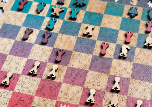
Our Wooden Chess Puzzle is both a jigsaw puzzle and playable chess game complete with board and pieces. After you’ve assembled this challenging…
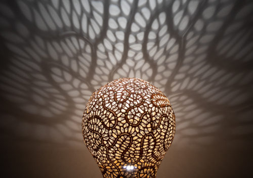
The Puzzle Cell Lamp is now available as a table lamp! You can order the table lamp version in our shop now. It…
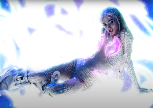
We collaborated with fashion designer Asher Levine to create a dragonfly wing inspired bodysuit for Grimes latest music video “Shinigami Eyes”. We worked with Asher…
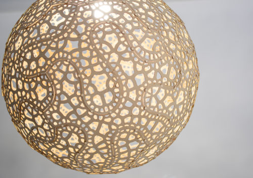
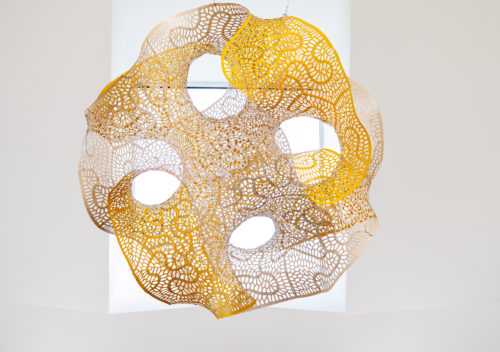
Finally! A new product from Nervous System that is not a jigsaw puzzle. Or is it? This otherworldly wood pendant lamp arrives at…
Baffling Bubbles is a brain bending wooden puzzle brought to you by Nervous System and artist Chris Yates. Each colorful bubble is a…
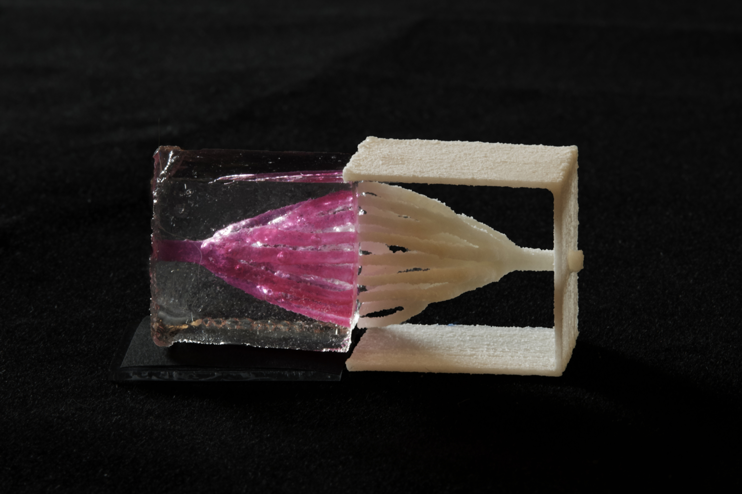
Nervous System collaborated with bioengineers at Rice University to create complex blood vessel networks using generative design and 3D-printed sugar. In a paper…